
EPR/81/INF. 7
September 1981


| FOOD AND AGRICULTURE ORGANIZATION OF THE UNITED NATIONS | ESN: FAO/WHO/UNU EPR/81/INF. 7 September 1981 |
| WORLD HEALTH ORGANIZATION | |
| THE UNITED NATIONS UNIVERSITY |
INFORMATION PAPER No. 7
Joint FAO/WHO/UNU Expert Consultation on
Energy and Protein Requirements
Rome, 5 to 17 October 1981
HUMAN PROTEIN REQUIREMENTS
AUTOCORRELATION AND ADAPTATION TO A LOW-PROTEIN DIET
CONTAINING
.356 GM PROTEIN/KG OR 57 MG N/KG BODY WEIGHT1–3
by
Ned Durkin, Dale A. Ogar, Shobha G. Tilve and
Sheldon Margen
University of California
Berkeley
ABSTRACT In order to test the model of protein deficiency proposed by Sukhatme and Margen (1), a 77-day metabolic study was carried out on 6 young men confined to a metabolic unit. They were fed an otherwise complete formula containing 57 mg N (.356 gm protein)/kg/day derived from egg albumen. Activity was programmed, and biochemical and physical performance were regularly monitored. The significant findings were: (1) By day 77 all 6 subjects had “adapted” or achieved balance (in a statistical stochastic sense). Some were in “slight positive balance”; others were in “slight negative balance”; but all were within the balance range. (2) All but one of the 6 subjects showed autocorrelations of nitrogen balance--with an exponential decay over time--after the steady state was achieved. This indicates to us that at this level of N intake the subjects were in a steady state and within the range of adequate nitrogen intake, thus demonstrating regulation and homeostasis. (3) Most of the subjects lost weight during the study. The rate of weight loss diminished as the experiment proceeded. The nature and significance of this remains unclear. (4) There were no demonstrable biochemical or physiological (work performance) changes, except for a marked fall in BUN. (5) The time required to reach a steady state varied from 7 to more than 28 days. The reasons for this variability are not clear. However, this calls into question the use of “short” metabolic periods to predict nitrogen requirements by the slope-intercept ratio. These findings make it necessary to question the methods and concepts currently used in defining protein requirements.
KEYWORDS Nitrogen balance, protein requirements and regulation, autoregulation, autocorrelations
Introduction
In spite of its great importance to individuals and society, neither the minimal nor the optimal level of human dietary protein intake has been clearly established. The literature reveals various definitions of “protein requirement,” usually based on several different conceptual or methodological approaches. The latest of these defines an adequate or “safe” level of protein intake, and thus attempts to avoid the issue (2). However, the terms “safe” and “recommended” are still used almost interchangeably, and so the confusion and contradiction remain (3).
In 1881, after looking at the diets of German workers, Voit recommended an intake of 118 grams protein per day for a 70 kg adult; in 1905 Chittenden estimated the requirement at less than half that by studying the intake of American soldiers and athletes (4). In 1920 Sherman (5) reviewed 109 experiments performed in Germany and America and noted a range of protein requirements from .3 to .93 gm/kg body weight. Although most of the experiments did not cite statistics, and it is not clear how Sherman analyzed them, it is nevertheless instructive to note his observations that the chief cause of variation was “the differing duration of the investigations and the differing extent to which the subject had accustomed himself to a low-protein diet” (5).
Although some of the discrepancies between so-called “safe” levels or requirements of populations or study cohorts can be attributed to the methodology used and the manner in which requirements are defined or conceptualized and interpreted, a more important reason for the continuing controversy may be the scarcity of long-term studies using low levels of protein. These are particularly important because only long-term studies can present conclusive evidence of adaptation and achievement of steady state which can be confirmed by subjecting the data to various types of time series analyses.
Although adaptation and the metabolic response to different levels of dietary protein have been studied extensively in animals (6, 7), little attention has been paid to the phenomenon in humans. Rather, the tendency has been to accept a concept of fixed minimum requirements as defined by current methodological techniques and not to realize that the individual is capable of adapting and achieving equilibrium (in the stochastic sense) at low levels of protein (8, 9).
The methodology and underlying assumptions used by the 1971 FAO/WHO Expert Committee in arriving at a so-called “safe” level of dietary protein have now come into question (2). Implicit in the Committee's recommendations are the following assumptions which deserve critical thought. (a) There is a required minimal level of protein intake, but no maximal level above which protein intake may be deleterious. A “safe” level should satisfy the needs of most (97.5%) individuals in a population rather than cover the average need. All are encouraged to eat at the “safe” level since eating below that level suggests a risk of protein deficiency. (b) The individual non-pregnant adult's requirement is genetically fixed over time in that there is inter- but not intra-individual variability. The concept of protein homeostasis or adaptation is not mentioned.5 (c) The “safe” level of protein is extrapolated from the slope intercept relating nitrogen balance to change in intake. (d) The obligatory nitrogen (N) loss (urine, feces, sweat, etc.) was used in hopes that this would define requirements. The Committee used an initial value of 54 mg N/kg body weight/day (as the average of the obligatory loss); this was increased by a factor of 30% (to 70 mg N/kg body weight/day) to correct for differences noted in the efficiency of utilization during short-term studies with a high quality protein (egg albumen). This added amount was necessary because, in short-term balance studies, simply replacing the N losses of individuals on a protein-free diet with high quality protein does not bring the subjects into balance. At N intakes slightly above the sum of factorial losses, the improvement in N balance was proportional to the protein added to the diet. When N intake was increased still further above the sum of obligatory losses and the level needed for N balance was approached, the efficiency of N utilization was reduced. The same 30% correction factor was used in setting the requirements for both adults and growing children. The Committee then increased this 70 mg N/kg body weight per day by another 30% (to 91 mg N/kg/day) to cover the requirements not only for an average individual but for 97.5% of all individuals within a given population. This latter 30%, which is equivalent to two standard deviations, is based on the 15% coefficient of variation observed in the obligatory N loss for the individuals on a protein-free diet. The fact that the intra-individual variation was as great as the inter-individual variation was ignored as a random methodological error. The factor 6.25 is used to convert the 91 mg N/kg/day to .57 gm protein/kg/day, the current recommended “safe” level. There is no empirical evidence to establish the validity of extrapolating from losses on a N-free diet to a “safe” level for a free-living population.
The report of this Expert Committee has been criticized by different people for very different reasons. Garza et al. (10) claim that the “safe” level is not sufficient to maintain long-term N balance in a significant number of healthy men. More recently, Sukhatme and Margen (1) have questioned the assumptions made in determining protein requirements and have proposed a new model for estimating protein deficiency. It is based on the observation that at fixed levels of N intake, an individual's daily N output does not fluctuate in a random manner but shows serial correlations. This means that there are cycles in nitrogen balance so that on some days high values for output tend to be followed by high values and on other days low values by low. Thus, today's nitrogen status will influence tomorrow's, but exert somewhat less of an influence on the-day-after-tomorrow's nitrogen status, and so on. This also means that today's requirement may differ from tomorrow's.
The statistical techniques used in the Sukhatme and Margen model were originally developed by engineers in order to detect and separate signal from noise when there is a high noise to signal ratio or even no signal at all. The model is stochastic in nature and is called autoregressive because it deals with a series of variables which are ordered in time. In autoregressive models the current value of the variable, such as UN or N balance, is regressed on the values for preceding days. This demonstrates an ordered (nonrandom) relationship between the variables over time. Serial correlations, Pk, will indicate the strength of the relationship for values on day x and day x-1, between day x and day x-2, and so on for different values of k.
Rand et al. (11) differ with Sukhatme and Margen and claim that the variations in UN output are random. In the random model favored by Rand et al. (11), there is no physiological regulation of N balance, so that when an individual is on a constant N diet for a series of days, there will be no serial correlation of UN output over time, and thus UN will be random. Symbolically, this can be expressed:
UN(d) = μ + ed
This means that the urinary nitrogen (UN) on any day (d) will correspond to the equilibrium value (μ) of output for the series plus the random error (ed) on that day. In the random model there is essentially all noise and no signal, so the error can be virtually eliminated by averaging over a sufficient number of days. Although the UN values differ, there will be no pattern to them and the variability can be ascribed to chance or measurement errors.
On the other hand, in a regulated system there will be a signal which will declare itself by showing serial- or auto-correlations. Such a pattern is consistent with homeostatic control. Thus, if an individual is on a constant N intake, the UN will not be random but will be autocorrelated. It can be expressed symbolically as:
UN(d) = μ + E(d)
where E(d) = ρ1[E(d-1)] + ρ2[E(d-2)] + … + e
In the model, μ still represents the average or equilibrium level of output for the series, but differs from the preceding function in that E is not random error. E is influenced by the value on the preceding days. The symbol ρ is a constant which is specific for an individual and relates the value of the UN on day d to the value on d-1, while ρ2 relates the value on day d to the value on d-2, or two preceding days. Thus, as we have said, the present value of UN will be influenced by the preceding day or days and exert influence on tomorrow's value. This becomes very important in structuring balance studies because in short-term experiments the carry-over of influence from one day to the next may obscure the value of a new treatment.
A characteristic feature of the autoregressive model is that ρd is equal to ρd. (This is a characteristic of a first-order autoregressive process and is referred to as Markovian.) The value of ρ2[E(d-2)] will be less than ρ1[E(d-1)] because ρ2[E(d-2)] equals ρ2[E(d-2)]. This follows because ρ is always less than 1, and ρd = ρd. It can be seen from the expressions that the value of ρk will decrease exponentially as the number of days preceding d increases; the separation of days is referred to as lag k. Stated another way, on day 1, ρ will represent the significant impact of UN or N balance on day 2's values, and the lesser impact on the values for day 3, etc. As the time interval increases and the value of ρ exponentially decreases, there will come a point when ρx will be small and there will be no significant effect of the values for day x on day 1. This fall-off or exponential decay of ρ with time is an essential feature of regulated systems.
Stationary variance is another feature of the model, and therefore the mean, covariance and variance of a series are independent of time and are constant. Thus, an individual's values for nitrogen balance and urinary nitrogen output should have a constant mean and standard deviation if the individual has achieved stationarity or a statistical steady state during the observed interval of time.
It should be clear that if the mean and variance are constant over an interval of time, no trend is present. These concepts are mentioned here because if the techniques of autocorrelation are to be applied appropriately, one has to insure that there is no trend. For example, if, as happens in our study, an individual switches from a moderate- or high-protein diet to a low-protein diet, the initial values for UN will consistently fall because of the reduction in protein intake and the initial adaptation to dietary change. Typically, the output on day 1 will be followed by a lower value on day 2, and a still lower value on day 3. This trend observed in the first days (or weeks) will give rise to significant autocorrelations and must be distinguished from the serial correlations observed after the individual has achieved equilibrium with a low but adequate protein intake. If there is a linear trend in the data, ρ will be significant but will not fall off exponentially. If the individual is in equilibrium, the mean, the standard deviations, and ρ will be constant for the interval of time being observed.
The presence of serial correlations implies that nitrogen, like energy, sodium, calcium and other elements of life, does not change in a random manner, but fluctuates within homeostatic limits and is subject to regulation. It further suggests that in the face of intra-individual variability, one cannot define the requirement but must rather speak of requirements within limits which will be satisfied by a range of intakes that maintain protein homeostasis.
The following study was undertaken to test the autocorrelation model and to see if an intake of 57 mg N/kg of body weight per day (.356 gm protein/kg body weight per day) could maintain protein homeostasis. Although this level of intake is only 62% of the FAO/WHO “safe” intake and significantly below the level found inadequate at MIT (11), previous work in this laboratory has shown that a considerable amount of adaptation to protein intake can take place. Although there are anecdotal reports of individuals on long-term low-protein diets (12), this is believed to be the longest controlled study at such a low level. Nitrogen level was kept constant throughout the study while minor adjustments in kilocalories (kcal) and activity levels were made during the first 18 days.
Materials and methods
Six men between the ages of 20 and 31 were selected from a large and varied applicant pool. The subjects included on Black, one Hispanic, and four Caucasians. All were free from any significant medical or physical abnormalities. Subject 5802, however, was 3-year postsplenectomy, secondary to a traffic accident. All had benign past medical histories and normal physical examinations, blood counts, serum chemistries, urinalyses, and electrocardiograms (see Tables 1, 2). All were negative for hepatitis B surface antigen and did not have antibodies to either the hepatitis B surface or core antigens.
Two of the men were lacto-ovo vegetarians (5803, 5805). The prestudy diets of all 6 men were determined by 3-day diet histories which were reviewed by an experienced dietitian and judged “adequate” with respect to protein and calories. The only possible exception was the diet of subject 5806 who had restricted his caloric intake during the preceding 6-month period and lost approximately 5 pounds.
The men were confined to the metabolic laboratory, known as the Penthouse, in the Department of Nutritional Sciences, from the evening of September 30 to the morning of December 18, 1980. They were allowed no visitors, but were able to communicate with the outside by telephone and mail. Prior to the onset of the study, all procedures used in this metabolic unit were reviewed and approved by the Committee for the Protection of Human Subjects at the University of California, Berkeley. Informed consent was obtained from each of the subjects and the study was carried out pursuant to DHHS guidelines. Although the subjects had the option to terminate their participation in the experiment at any time, all 6 remained throughout the 77-day period.
Diet. The composition of the diet, which was similar to that used in previous Penthouse studies, is shown in Table 3. The basic formula was the same for all 6 subjects. However, protein intake was individually adjusted to .57 mg N/kg (.356 gm protein/kg) initial body weight by adding an egg albumen solution to the basic formula, and calories were likewise adjusted by the addition of an extra-calorie solution. Caloric adjustments were made on a trial and error basis during the first 17 days of the study with the hope of stabilizing body weight (Table 4). In addition to the liquid formula diet, which was served in equal amounts four times each day, instant decaffeinated coffee and instant tea were served at alternate meals; frozen peaches were served at one meal per day; low-protein rusks at another. Vitamins, choline, and trace minerals (without iron, copper, and zinc) were taken daily in pill or capsule form. A solution of iron, copper, and zinc was added back into the formula in order to facilitate an ancillary study on stable isotope absorption which will be reported elsewhere. Deionized water was available ad libitum after a required minimum intake of 1,000 m1/day.
Either a dietitian, a dietitian's aide, or a registered nurse was present at all meals to insure complete consumption of the diet. Meals were served at 8:30 a.m. and 12:30, 4:30 and 8:30 p.m. Actual levels of N and kcal were checked by composite analysis four times throughout the study.
Experimental procedures. Prior to arising at 8:00 a.m. each subject had his temperature, pulse and respiratory rate taken. Subjects were then asked to void and weigh themselves wearing only their undershorts. Urine and feces were collected daily as voided according to strict protocols and analyzed in the established manner (13). Urinary nitrogen was determined by the micro-Kjeldahl method, creatinine by the automated picrate method. Fecal output was pooled and analyzed for nitrogen. The pool periods were days 6–14, 15–35, 36–56, and 57–77 (Table 5).
Each subject had two organized exercise periods per day which consisted of alternate 20–30 minute periods on a bicycle ergometer and a treadmill. They were able to choose their activity level, and minor changes were permitted during the first 17 days. However, from day 18 through the end of the study, formal exercise remained constant. The individual activity levels are shown in Table 6. Other daily activities were according to personal preference within the limits set by the experimental protocol, i.e., no sunbathing and no activities that required leaving the unit. Much of the subjects' free time was spent in generally sedentary activities, reading, watching television, and playing pool. The day ended at 11:00 p.m.
Each subject was given three fitness tests: the first on day 13 or 14, the second on day 40 or 41, and the final one on day 65 or 66. During the test, each subject rode a bicycle ergometer for 6 minutes at loads of 200, 400, 600, 800, and 1,000 kg.m/min, separated by 5-minute rest periods. Heart rate (from EKG), O2 consumption and CO2 production were determined during the final two minutes of each exercise period.
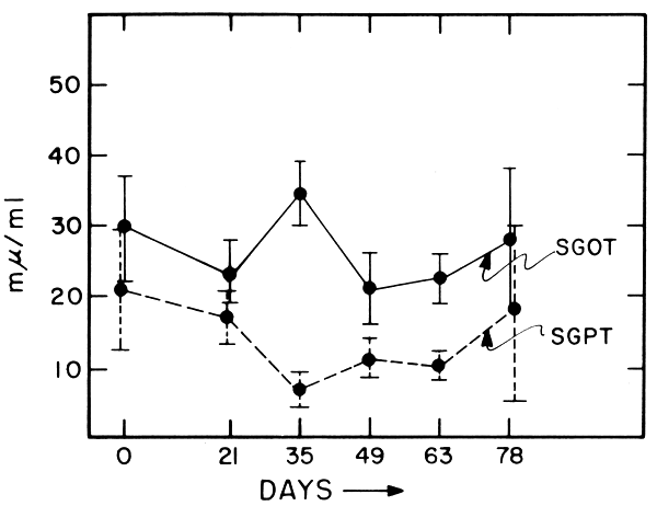
Because of the possibility of changes in liver chemistry, serum enzymes were monitored on days 21, 35, 44, 63 and 78. Fasting blood was drawn from the antecubital vein into tared vacutainer tubes which were then reweighed, centrifuged and analyzed. Hair samples were obtained periodically during the experiment and examined for morphological changes by Dr. Robert Bradfield. These results will be reported elsewhere.
Results
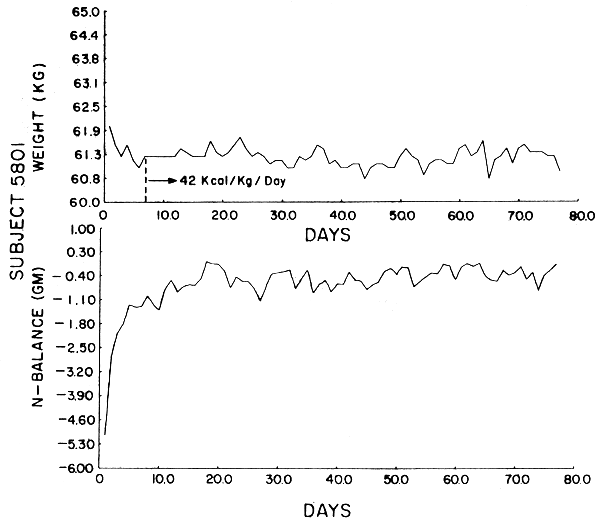
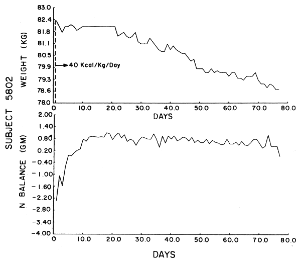
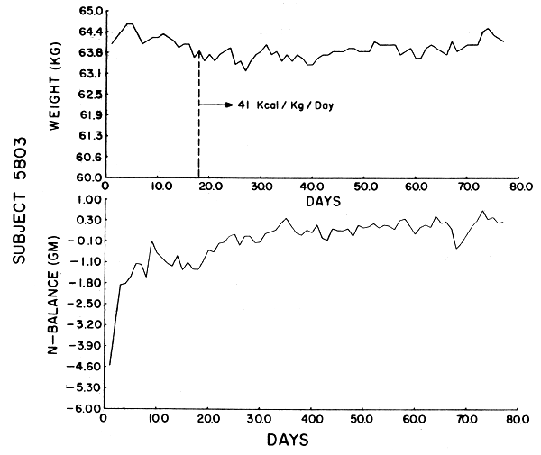
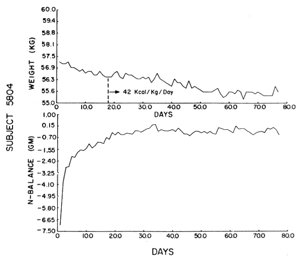
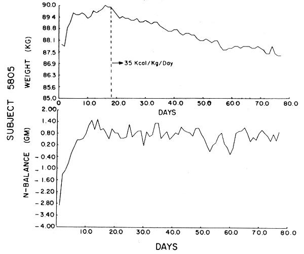
The data were analyzed by computer using the Statistical Package for the Social Sciences (SPSS). Figures 1–6 show the weight in kg, the amount of kcals fed, and the apparent N balance for each subject over the 77 days of the study. Nitrogen balance is crude in that it represents the sum of urinary and stool losses but ignores minor miscellaneous losses such as sweat, breath, etc. The fecal losses for each collection period were used in calculating the N balance for that period. Nitrogen intake is 57 mg N/kg/day x initial body weight in kg (see Table 4).
Tables 7–12 display the values for ρ which represent the relationship between the values at increasing numbers of days. The entire series, as well as the series after successively eliminating one week at a time up to the fourth week, was subject to analysis. Both UN and N balance were analyzed in the same way. By arbitrarily dividing the experimental period into five groups, namely days 1–77, 8–77, 15–77, 22–77, and 29–77, it is possible to see when a steady state is achieved, both in terms of ρ and UN or N balance.
A brief resume of the results follows for each subject.
Subject 5801. This subject lost a total of .8 kg over the 77 days, half of which he lost after the first two weeks. By laboratory analysis he received 3.68 gm N/day. His UN series was highly correlated, but because of the continuous trend in UN output, which decreased throughout the study, it did not show the exponential drop-off. When N balance is considered, the subject achieved a steady state after two weeks and showed significant autocorrelation with an exponential decay. The subject showed a consistent increase in stool N output over time. Although he showed a slightly negative balance throughout the study, he was in “balance” on the final day. All laboratory work was within normal limits except for BUN, and there was no deterioration of fitness.
Subject 5802. He received 4.96 gm N/day. For the first three weeks of the study he maintained the most constant weight of all the subjects and yet had the largest overall weight loss (3.9 kg), most of it occuring after the third week. The subject was in positive balance within 10 days, but showed a trend toward balance. This was reflected in the high serial correlations for UN and N balance which did not decrease exponentially. All laboratory work, except BUN, was again within the normal range and there was no fall-off in work efficiency.
Subject 5803. This subject received 3.82 gm N/day. He gained .3 kg over the 77 days but had a weight change of +.4 kg from day 22–77. His trend toward positive balance lasted for 21 days, after which time he achieved a steady state. He was in borderline positive balance soon after that and remained so for most of the rest of the study. After stationarity was achieved, his UN and N balance showed a high degree of autocorrelation and the expected exponential decrease in ρ. His laboratory work was within normal limits with the exception of a low BUN, an albumin which was .1 gm/d1 above the reference range, an SGOT 3 units above, and an SGPT 4 units above the reference range (all well within the normal bounds of laboratory variability). There was no deterioration in fitness.
Subject 5804. This subject received only 3.43 gm N/day. He lost a total of 2 kg over 77 days, .8 kg of which was after day 21. He achieved stationarity after 21 days when his trend toward positive balance stabilized. After that time he was generally in borderline negative balance. He had achieved a steady state, however, in that after day 22 his UN and N balance values were correlated and showed the expected exponential decline. His final laboratory values were normal. There was no fall-off of work efficiency.
Subject 5805. Subject 5805 received 5.25 gm N/day and had a weight loss of .6 kg over the entire study. However, after a rapid weight gain in the first week of the study, he lost a total of 2.30 kg from day 8–77. The subject achieved stationarity in one week and was also in significant positive balance at the end of one week. He remained so for the rest of the period. Both his UN and N balance showed autocorrelations and exponential decline of ρ after one week. All laboratory values, except for the final BUN, were within the reference range.
Subject 5806. Subject 5806 received 5.3 gm N/day, lost 2.6 kg over the 77 days and .9 kg from day 29–77. He did not achieve stationarity during the initial 28 days, but did so after that. His UN and N balance values were highly correlated, with the exponential decline showing itself after 29 days. With the exception of a low final BUN, all laboratory work was within the reference range and there was no deterioration of work efficiency.
Liver enzymes for all 6 subjects were measured frequently during the study and were within the normal range, so it is quite unlikely that any elevations were missed. Although an analysis of variance showed significant changes during the study (Table 13; Figure 7), there were no trends and the changes were less than frequently seen in our studies on free-living populations (14).
Discussion
The data presented in this study are clear and compelling evidence that our present concepts of protein requirements must be drastically revised. Certainly, it is no longer possible to speak of a “fixed” daily requirement for protein. Any attempt to define an individual's protein requirement must be done in a dynamic context which allows for adaptation. Of equal importance is the fact that the balance data on the “low protein” diet of .35 gm protein/kg body weight differ so strikingly and significantly from previously published work (2, 10, 15). that concerns about the FAO/WHO “safe” level being inadequate are not warranted. Furthermore, statistical analysis shows that UN and N balances are usually autocorrelated, confirming the hypothesis of Sukhatme and Margen. This reinforces the homeostatic nature of N balance and may lead to a model which defines the upper and lower limits of optimal protein intake.
The outcome of this study has many implications. A different conceptualization of the protein requirement will not suffice if it is not accompanied by a search for better methodologies to define the requirement. Both the factorial method and the slope intercept are static techniques and cannot be used to define a requirement that is changing. Even in the “adapted” state the requirement varies from day to day, as evidenced by the autocorrelation data. Regardless of the interpretation of these results, it should be apparent that the actual “protein requirement” is significantly less than previously supposed.
Confinement and control of subjects is probably the single most important methodological difference distinguishing our work from that done at MIT and may explain some of the differences between our data and theirs. This more rigorous control of confounding variables prevents the signal from being swamped by the noise.
The study used crude N balance in that sweat and other miscellaneous losses were not measured. Because of the low levels of dietary protein and the compensatory fall in BUN, nitrogen losses in the sweat would be substantially below the FAO figures and thus could not significantly alter the N balance data. The difference between being “in balance” or not being in balance is small and within the range of “experimental balance” (and certainly in balance or approaching such in a stochastic sense). The search for the ephemeral “zero” balance must be brought to a halt; there is only a statistical zero balance with some variability.
It should be reassuring to note that all 6 subjects tolerated the diet well. There were few significant changes in biochemical parameters or ability to do work. All were either in balance or close to being in balance at the end of the study. This is all the more remarkable because the level of calories fed was considerably lower than that used in other studies (10, 15). Five of the six subjects lost weight, though only 3 of those lost 2 or more kilograms. If anything, it is likely that N balance might have been improved if calories had been increased so that body weight was maintained. However, the fact that a “steady state” occurred in most subjects even under these conditions is important. A subsequent paper will examine autocorrelation and N balance with a more generous level of calories.
The present study is considered to be long-term, though in reality 77 days is a short time in the life of an adult. There is no way of knowing what constitutes an adequate length of time for a study such as this. Some subjects adapt within a few days; others require 28 days. It appears that Subject 5802 was in the process of adapting throughout the 77 days. He exhibited a continuous trend and had not reached a steady state at the end of the experiment. This is a possible explanation for the failure of his UN or N balance series to show the exponential decay in autocorrelation. It is interesting that subject 5801 showed a significant autocorrelation, with exponential decay, in N balance but not UN. This subject showed an increase in fecal N over time. The fact that autocorrelation was observed when N balance was analyzed may be a random finding but may also indicate that the gut cannot be ignored when speaking of total N regulation. There are no data or clues to suggest why some adapt so much more quickly than others. The idea that a period of 10 days is adequate for adaptation goes back to studies using a protein-free diet where UN was found to fall and apparently plateau after 10–18 days (13, 17). It should be obvious that the apparent stability of UN on a protein-free diet cannot be used to justify a period of 10–18 days for determining the adequacy of different levels of dietary protein. Clearly, the data obtained by removing protein from the diet cannot be used to justify the length of an experiment containing protein. Furthermore, careful analysis of our data on protein-free diets still shows a trend in a significant number of subjects (personal analysis).
It should be noted that after reaching equilibrium, at least 35 days of data are needed to apply the statistical techniques of autocorrelation. The data also demonstrate problems in the way nitrogen or protein requirement is expressed. Traditionally, they have been expressed on a mg/kg-body-weight basis. There is a certain inequity in this method, for it assumes that a kg of body weight is of similar composition in different healthy individuals. The most extreme example of this can be found in a comparison of Subjects 5804 and 5806. Subject 5806 was only 1.3 cm taller than 5804 but was initially 30.9 kg heavier. By weight-for-height and body-mass-index (BMI) (kg/m2) standards he (5806) was slightly overweight, but clearly not obese. Both had similar kcal from protein/total kcal ratios, but 5806 received 11 gm (52.7%) more protein than 5804. Subject 5804 lost 2 kg over the 77 days and only approached balance; 5806 lost 2.6 kg and was in positive balance. This is a clear example of why N “requirements” should better be expressed as a function of lean body mass or other parameters of active tissue rather than total body weight. This would recognize the significant normal variation of body composition within a healthy population, and would acknowledge the fact that it is the lean body tissue--not the adipose tissue--which requires the bulk of the dietary nitrogen.
Although this discrepancy between N required by total body weight and lean body mass is important, it cannot explain several other puzzling phenomena. For example, Subjects 5805 and 5806 are similar in height, weight and BMI. Subject 5805 received 5.24 gm N and was in positive balance within one week. Subject 5806 received 5.35 gm N and was not in balance until some time after the 28th day, and Subject 5802 demonstrated a trend for 77 days. We cannot explain this large variation in the rate of adaptation. It should be clear, though, by examining Table 14 that all 6 subjects were using N more efficiently in the last 6 days than they were in days 5–10. Although the ability to adapt is clearly beneficial to the individual, it is not clear that the adapted state is ideal. There are no data to suggest that a specific level of intake is optimal. At present, all that can be suggested is that a range of intakes can be defined.
By examining the serial correlations of the 6 subjects, several things should be clear. Generally, the correlations for UN and N balance are of similar magnitude in the subjects. The correlations show the nonrandom notion of N balance and clearly are different from those of Rand et al. (11). The cyclic nature of N balance is perhaps most easily appreciated by examining this apparent N balance of Subject 5805 from day 45–77 (Figure 5). These significant correlations support the concept of regulation. It should be pointed out though, even if there were no serial correlations, the homeostatic nature of protein metabolism is clear.
The question has been raised as to why we did not measure body composition in these studies. The answer is that the measurement errors of any of the available methods, at least in our hands, are too great to have allowed for interpretation of expected or observed changes. The weight changes are puzzling and we wish that we could explain them. Four subjects lost weight, but the loss seemed to be decreasing with time. It is not clear whether this was part of the adaptation or was related to changes in energy balance. It could not be related to changes in N balance.
We feel that the data presented here have significant policy implications. Although care must be taken in extrapolating work done with young healthy men to populations who live outside a temperate hygienic metabolic unit, it is nevertheless necessary to do so. Morley and Chang (17) have recently shown that nutritionists in developing countries still insist on promoting protein-rich foods and have ignored the work of Sukhatme (18) who has shown that protein deficiency is secondary to a deficiency of the food habitually eaten. There is a “food gap”--not a protein gap. In this study, protein provided between 3.39 and 4.07% of calories. From the viewpoint of policy, it does not appear to be prudent to push for protein supplements or protein-dense foods.
Another policy implication relates to the FAO/WHO Expert Committee recommendations. It can be stated with certainty that eating below the FAO/WHO safe level of 91 mg N/kg does not necessarily imply a risk of protein deficiency. Obviously, eating less than a certain level of protein may be harmful and beyond the adaptive powers of the individual. It is not the intent of this paper to promote .57 mg N/kg or .35 gm protein/kg body weight as the new “safe” level or suggest that it is the lowest limit of acceptable intake. We do not know what that lower limit is. There also may be an upper level of protein intake which is beyond adaptation. Earlier work using the techniques of autocorrelation have shown that at high levels of intake the homeostatic pattern is interrupted and N balance fluctuates wildly in a random manner (19). All this work suggests that N requirement be defined within a range in order to recognize and correctly interpret intra-individual variation. This allows for accepting and incorporating the concepts of adaptation and homeostasis in N metabolism. New analytical techniques will have to be used to define these limits, but it should be clear that extrapolations from N losses on a protein-free diet or the slope intercept technique are not adequate.
In addition, more work needs to be done with individuals eating their habitual diets and performing their usual activities. Adaptation is not limited to protein requirement and may well require more time than can be used in metabolic unit studies. It seems that the best way to provide data useful for developing countries is to generate the data in those countries.
In conclusion, 6 men adapted to and tolerated a diet containing 57 mg N/kg or .35 gm protein/kg. N balance and UN were autocorrelated, confirming the controlled nature of these phenomena.
References
Sukhatme PV, Margen S. Models for protein deficiency. Amer J Clin Nutr 1978;31:1237–1256.
World Health Organization. Energy and protein requirements. Report of a joint FAO/WHO ad hoc expert committee. Geneva: WHO, 1973 (WHO Tech Rep Ser No. 522, FAO Nutr Meet Rep Ser No. 52).
Committee on Dietary Allowances, Food and Nutrition Board, National Research Council. Recommended dietary allowances. 9th revised ed. Washington, DC: National Academy of Sciences, 1980.
Chittenden RH. Physiological economy in nutrition. New York: FA Stokes Co, 1980, 1905.
Sherman HC. Protein requirement of maintenance in man and the nutritive efficiency of bread protein. J Biol 1920;41:97–109.
Durkin EJ, Nishikawara MT. Effect of starvation, dietary protein and partial hepatectomy on rat liver, aspartate and ornithine carboamyl transferases. J Nutr 1971;101:1457–1474.
Schimke RT. Adaptive characteristics of urea cycle enzymes in the rat. J Biol Chem 1962;237:459–468.
Waterlow JC. Observation on the mechanism of adaptation to low protein intakes. Lancet 1968;II:1091–1097.
Gopalan C. Adaptation to low calorie and low protein intake: does it exist. In: Margen S, Ogar RA, eds. Prog Hum Nutr 1978;2:132– 141.
Garza C, Scrimshaw NS, Young VR. Human protein requirements: a long-term metabolic nitrogen balance study in young men to evaluate the 1973 FAO/WHO safe level of egg protein intake. J Nutr 1977; 107:335–352.
Rand WM, Scrimshaw NS, Young VR. Analysis of temporal patterns in urinary nitrogen excretion of young adults receiving constant diets at two nitrogen intakes for 8–11 weeks. Amer J Clin Nutr 1979;32: 1408–1414.
Strieck F. Metabolic studies in a man who lived for years on a minimum protein diet. Ann Intern Med 1937–1938;11:643–650.
Calloway DH, Margen S. Variation in endogenous nitrogen excretion and dietary nitrogen utilization as determinants of human protein requirement. J Nutr 1971;101:205–216.
Personal observations.
Garza C, Scrimshaw NS, Young VR. Human protein requirements: evaluation of the 1973 FAO/WHO safe level of protein intake for young men at high energy intakes. J Nutr 1977;37:403–420.
Scrimshaw NS, Hussein MA, Murray E, Rand WM, Young VR. Protein requirement of man: variations in obligatory urinary and fecal nitrogen losses in young men. J Nutr 1972;102:1595–1604.
Morley D, Chang CY. Inappropriate nutrition education in the villages. Lancet 1981;I:209.
Sukhatme PV. The protein problem: its size and nature. J Royal Statist Soc 1974;137:166–191.
Oddoye EA, Margen S. Nitrogen balance studies in humans: long-term effect of high nitrogen intake on nitrogen accretion. J Nutr 1979;109:363–377.
Footnotes
Supported in part by Grants AM10202 and AM07155 from the National Institute of Arthritis, Metabolism and Digestive Diseases.
Address reprint requests to: Sheldon Margen, M.D., School of Public Health, University of California, Berkeley, CA 94720.
Present address: Maharashtra Association for the Cultivation of Science, Law College Road, Poona, India.
TABLE 1
Characteristics of the men
| Subject No. | Age | Height | Initial weight | Body mass index | Weight change |
|---|---|---|---|---|---|
| yr | cm | kg | kg/m2 | kg | |
| 5801 | 28 | 181.2 | 62.6 | 19.06 | -0.8 |
| 5802 | 29 | 181.5 | 84.2 | 25.56 | -3.9 |
| 5803 | 31 | 175.3 | 64.8 | 21.09 | +0.3 |
| 5804 | 22 | 180.2 | 58.6 | 18.03 | -2.0 |
| 5805 | 30 | 190.4 | 89.1 | 24.57 | -0.6 |
| 5806 | 27 | 181.5 | 89.5 | 27.17 | -2.6 |
TABLE 2
Summary of initial (i) and final (f) laboratory values
| Parameter | Subject Number | |||||||||||
|---|---|---|---|---|---|---|---|---|---|---|---|---|
| 5801 | 5802 | 5803 | 5804 | 5805 | 5806 | |||||||
| i | f | i | f | i | f | i | f | i | f | i | f | |
| Total protein, gm/dl (6.0–8.3)* | 6.9 | 7.2 | 7.1 | 7.5 | 8.0 | 8.1 | 7.4 | 7.6 | 7.3 | 7.1 | 7.2 | 7.4 |
| Albumin, gm/dl (3.5–5.1) | 4.2 | 4.5 | 4.0 | 4.8 | 4.6 | 5.2† | 4.7 | 5.3† | 4.6 | 5 | 4.2 | 4.2 |
| BUN, mg/dl (6–25) | 12 | 3† | 10 | 5† | 9 | 2† | 15 | 6 | 10 | 4† | 11 | 5† |
| SGOT, mu/ml (8–45) | 24 | 29 | 37 | 23 | 37 | 48† | 18 | 26 | 32 | 26 | 31 | 17 |
| SGPT, mu/ml (3–40) | 13 | 12 | 24 | 5 | 33 | 44† | 11 | 24 | 25 | 11 | 24 | 14 |
| GGT, mu/ml (7–51) | 18 | 15 | 35 | 16 | 16 | 22 | 11 | 13 | 20 | 18 | 15 | 21 |
| LDH, mu/ml (104–235) | 134 | 159 | 168 | 180 | 181 | 198 | 163 | 175 | 156 | 148 | 170 | 143 |
| Creatinine, mg/dl (0.5–2.0) | 0.8 | 0.9 | 1.0 | 0.9 | 0.9 | 0.9 | 0.9 | 0.9 | 0.7 | 0.8 | 1.1 | 0.9 |
| HCT, % (37–52) | 47.3 | 42.7 | 46.8 | 43.4 | 44.7 | 44.1 | 45.9 | 44.1 | 46.9 | 46.7 | 47.2 | 46.0 |
| Hemoglobin, gm/dl (12–18) | 16.2 | 15.0 | 16.0 | 14.6 | 15.2 | 15.1 | 16.2 | 15.1 | 16.5 | 15.7 | 16.3 | 15.7 |
| RBC count, 106/mm3 (4.2–6.2) | 5.3 | 5.07 | 5.17 | 4.96 | 5.06 | 4.95 | 5.2 | 4.96 | 5.42 | 5.49 | 5.47 | 5.37 |
| WBC, 103/mm3 (4.8–10.8) | 7.5 | 6.9 | 7.5 | 6.8 | 5.6 | 5.3 | 5.6 | 3.9† | 5.5 | 5.6 | 6.5 | 6.8 |
| Segs, % (50–70) | 61 | 64 | 38 | 43 | 40 | 48 | 57 | 44 | 59 | 51 | 66 | 66 |
| Lymphs, % (20–40) | 35 | 29 | 49 | 50 | 49 | 46 | 43 | 51 | 34 | 31 | 22 | 25 |
| Monos, % (2–10) | 1 | 4 | 6 | 5 | 3 | 3 | 2 | 4 | 3 | 1 | 1 | |
| Eos, % (1–4) | 3 | 5 | 1 | 8 | 3 | 27 | 1 | 3 | 5 | 12 | 9 | |
| Basos, % (0–2) | 1 | 2 | 1 | 10.4 | 2 | 1 | ||||||
| T3 uptake, % (25–35) | 28 | 27 | 30 | 26 | 27 | 27 | 2.9 | 25 | 27 | 26 | 33 | 25 |
| T4, μg/dl (4.2–12.5) | 7.1 | 7.6 | 7.8 | 7.5 | 6.1 | 6.6 | 10.1 | 7.6 | 8.2 | 7.1 | 7.3 | |
| Free thyroxine index | 2.0 | 2.1 | 2.4 | 1.9 | 1.7 | 1.8 | 2.5 | 2.1 | 2.2 | 1.9 | 1.9 | |
* Reference values in parentheses.
† Values outside of reference range.
TABLE 3
Diet composition
| Basic Formula (gm/subject/day) | |
|---|---|
| Egg albumen, dried | 17.788 |
| Maltodextrins | 111.945 |
| Cornstarch | 111.945 |
| Sucrose | 22.389 |
| Cottonseed oil | 13.609 |
| Shortening | 38.786 |
| NaCl | 3.556 |
| KCl | 4.444 |
| CaCO3 | .765 |
| Ca(H2PO4)2.H2O | 2.568 |
| MgO | .489 |
| Methylcellulose | 3.000 |
| Biotin | .0002 |
| Deionized water | 268.720 |
| Total | 600.000 gm |
| (150 gm/meal) | |
| FeCl3.6H2O | 25.52 gm/day → 10 mg Fe/day |
| CuSO4 | 4.43 gm/day → 3 mg Cu/day |
| ZnSO4.7H2O | 40.31 gm/day → 15 mg Zn/day |
| Cornstarch | 2.0 |
| Maltodextrins | 2.0 |
| Sucrose | .5 |
| Cottonseed oil | 1.0 |
| Deionized water | 7.4 |
| Total | 12.9 ml |
| (Supplement added to basic formula in varying quantities from days 1–17 to maintain weight. From days 18–77 amount remained constant.) | |
| Egg albumen, dried | 1 gm |
| Deionized water | 2 gm |
| (1 gm egg albumen solution contained 42.27 mg N; solution added to basic formula to bring N level fed to 57 mg/kg.) | |
| Low protein rusks | 22 |
| Frozen peaches | 100 |
| Instant tea | 1 |
| Instant decaffeinated coffee | 6.66 |
TABLE 4
Protein and energy intake
| Subject no. | Study days | Kcal/kg | Kcal/day | Total protein intake/day | Calculated N intake* | Non-protein N from extra kcal solution | Calculated total N intake | Laboratory analysis of total N intake† | Kcal from protein/total kcal |
|---|---|---|---|---|---|---|---|---|---|
| gm | gm | gm | gm | % | |||||
| 5801 | 1–6 | 40 | 2502.4 | 22.31 | 3.57 | .08 | 3.65 | 3.68 ±.03 | 3.40 |
| 7–77 | 42 | 2627.5 | |||||||
| 5802 | 1–77 | 40 | 3368.0 | 30.00 | 4.80 | .13 | 4.93 | 4.96 ±.05 | 3.56 |
| 5803 | 1–17 | 40 | 2590.0 | 23.06 | 3.69 | .08 | 3.77 | 3.82 ±.06 | 3.47 |
| 18–77 | 41 | 2654.8 | |||||||
| 5804 | 1–14 | 40 | 2344.0 | 20.88 | 3.34 | .06 | 3.40 | 3.43 ±.04 | 3.40 |
| 15–77 | 41 | 2402.6 | |||||||
| 18–77 | 42 | 2461.2 | |||||||
| 5805 | 1–6 | 40 | 3564.0 | 31.75 | 5.08 | .11 | 5.19 | 5.24 ±.04 | 4.07 |
| 7–14 | 38 | 3385.8 | |||||||
| 15–77 | 36 | 3207.6 | |||||||
| 18–77 | 35 | 3118.5 | |||||||
| 5806 | 1–9 | 40 | 3580.0 | 31.88 | 5.10 | .17 | 5.27 | 5.30 ±.07 | 3.39 |
| 10–77 | 42 | 3759.0 |
* 57 mg N/kg body weight.
† Mean of 4 values ± standard deviation.
TABLE 5
Fecal N (gm/24 hr): Average of 4 analyses of
2 samples from pool (range of 8 samples)
| 5801 | 5802 | 5803 | 5804 | 5805 | 5806 | |
|---|---|---|---|---|---|---|
| Day 6–14 | .346 | 1.070 | .664 | .692 | .826 | 1.016 |
| (.342–.351) | (1.058–1.085) | (.655–.675) | (.673–.705) | (.815–.835) | (1.011–1.024) | |
| Day 15–35 | .391 | 1.000 | .714 | .700 | .812 | .896 |
| (.389–.395) | (.993–1.012) | (.705–.720) | (.695–.713) | (.798–.876) | (.888–.904) | |
| Day 35–56 | .523 | .891 | .753 | .730 | 1.065 | .918 |
| (.516–.527) | (.886–.895) | (.745–.758) | (.724–.733) | (1.055–1.078) | (.916–.921) | |
| Day 56–77 | .577 | .858 | .577 | .808 | .816 | .863 |
| (.570–.583) | (.850–.859) | (.572–.578) | (.805–.812) | (.807–.825) | (.860–.868) |
TABLE 6
Individual formal exercise regimen
| Subject no. | Bicycle ergometer | Treadmill | |||
|---|---|---|---|---|---|
| kg.m/min | minutes | mph | grade | minutes | |
| % | |||||
| 5801 | 500 | 20 | 3.5 | 10 | 20 |
| 5802 | 1200 | 25 | 4.2 | 10 | 20 |
| 5803 | 500 | 20 | 3 | 10 | 20 |
| 5804 | 600 | 15 | 3 | 10 | 15 |
| 800 | 5 | 6 | 10 | 5 | |
| 5805 | 700 | 25 | 4 | 12 | 20 |
| 5806 | 700 | 20 | 4 | 10 | 20 |
TABLE 7
Subject 5801
| Values of | Daily UN series | N-balance series | ||||||||
|---|---|---|---|---|---|---|---|---|---|---|
| 1–77 | 8–77 | 15–77 | 22–77 | 29–77 | 1–77 | 8–77 | 15–77 | 22–77 | 29–77 | |
| N | 77 | 70 | 63 | 56 | 49 | 77 | 70 | 63 | 56 | 49 |
| Mean | 3.81 | 3.64 | 3.58 | 3.58 | 3.52 | -.63 | -.47 | -.41 | -.43 | -.39 |
| S.D. | .7440 | .3615 | .3026 | .3057 | .2744 | .69 | .31 | .26 | .26 | .24 |
| C.V. (%) | 19.5 | 10 | 8.5 | 8.5 | 7.8 | |||||
| p1 | .6180 | .6592 | .5541 | .5564 | .4907 | .5782 | .5483 | .4203 | .3946 | .3293 |
| p2 | .4695 | .4515 | .3378 | .3968 | .3566 | .4172 | .2922 | .1568 | .1902 | .1716 |
| p3 | .3951 | .3511 | .2494 | .3501 | .3418 | .3383 | .1750 | .0416 | .1291 | .1578 |
| p4 | .3083 | .2543 | .1624 | .2626 | .2435 | .2445 | .0579 | -.0788 | .0179 | .0436 |
| p5 | .2974 | .2584 | .2299 | .2942 | .2425 | .2372 | .0809 | .0100 | .0816 | .0604 |
| p6 | .2894 | .2799 | .3241 | .2323 | .1286 | .1276 | .2296 | |||
| p7 | .2390 | .2032 | .2758 | .1832 | .0608 | .1004 | .2274 | |||
TABLE 8
Subject 5802
| Values of | Daily UN series | N-balance series | ||||||||
|---|---|---|---|---|---|---|---|---|---|---|
| 1–77 | 8–77 | 15–77 | 22–77 | 29–77 | 1–77 | 8–77 | 15–77 | 22–77 | 29–77 | |
| N | 77 | 70 | 63 | 56 | 49 | 77 | 70 | 63 | 56 | 49 |
| Mean | 3.4290 | 3.3170 | 3.33 | 3.36 | 3.32 | .56 | .70 | .70 | .68 | .66 |
| S.D. | .4894 | .2562 | .2495 | .2355 | .2260 | |||||
| C.V. (%) | 14.3 | 7.6 | 7.5 | 7. | 6.7 | |||||
| p1 | .6193 | .5038 | .4797 | .3548 | .3258 | .6587 | .3525 | .3218 | .2103 | .2027 |
| p2 | .5016 | .4496 | .4486 | .3425 | .3066 | .5853 | .2785 | .2976 | .2139 | .2056 |
| p3 | .4223 | .4399 | .4483 | .2937 | .2912 | .4002 | .2859 | .3174 | .1800 | .2166 |
| p4 | .2831 | .3325 | .3318 | .2088 | .1910 | .2750 | .1459 | .1806 | .0809 | .1092 |
| p5 | .2702 | .4352 | .4408 | .3566 | .3607 | .2537 | .2766 | .3261 | .2585 | .3090 |
| p6 | .1765 | .3482 | ||||||||
| p7 | .1125 | .2992 | ||||||||
TABLE 9
Subject 5803
| Values of | Daily UN series | N-balance series | ||||||||
|---|---|---|---|---|---|---|---|---|---|---|
| 1–77 | 8–77 | 15–77 | 22–77 | 29–77 | 1–77 | 8–77 | 15–77 | 22–77 | 29–77 | |
| N | 77 | 70 | 63 | 56 | 49 | 77 | 70 | 63 | 56 | 49 |
| Mean | 3.47 | 3.29 | 3.20 | 3.08 | 3.03 | -.39 | -.21 | -.12 | .003 | .05 |
| S.D. | .82 | .5018 | .4261 | .26 | .24 | .82 | .51 | .44 | .27 | .26 |
| C.V. (%) | 24 | 15.2 | 13.3 | 8.4 | 8 | |||||
| p1 | .7385 | .7837 | .7857 | .5877 | .5259 | .7382 | .7873 | .7931 | .6196 | .5564 |
| p2 | .5845 | .7373 | .6439 | .3138 | .1804 | .5829 | .7367 | .6507 | .3521 | .2151 |
| p3 | .5300 | .6631 | .4923 | .1372 | -.0824 | .5279 | .6632 | .5049 | .1903 | -.0251 |
| p4 | .4539 | .5790 | .3211 | -.060 | -.3188 | .4517 | .5816 | .3439 | .0196 | -.2420 |
| p5 | .3978 | .5276 | .2268 | -.1374 | -.3189 | .3961 | .5360 | .2573 | -.0406 | -.2244 |
| p6 | .3833 | .4494 | .1900 | -.0981 | .3826 | .4627 | .2283 | .0148 | ||
| p7 | .3666 | .4402 | .1629 | -.0325 | .3647 | .4510 | .0500 | |||
TABLE 10
Subject 5804
| Values of | Daily UN series | N-balance series | ||||||||
|---|---|---|---|---|---|---|---|---|---|---|
| 1–77 | 8–77 | 15–77 | 22–77 | 29–77 | 1–77 | 8–77 | 15–77 | 22–77 | 29–77 | |
| N | 77 | 70 | 63 | 56 | 49 | 77 | 70 | 63 | 56 | 49 |
| Mean | 3.32 | 3.1 | 2.94 | 2.88 | 2.85 | -.64 | -.38 | -.27 | -.22 | -.19 |
| S.D. | 1.06 | .44 | .2671 | .1942 | .19 | 1.04 | .413 | .25 | .18 | .18 |
| C.V. (%) | 32 | 14 | 9.1 | 6.7 | 6.5 | |||||
| p1 | .6781 | .8378 | .6538 | .5381 | .4749 | .6691 | .8242 | .6138 | .4923 | .4462 |
| p2 | .5556 | .7648 | .4774 | .3201 | .2459 | .5438 | .7150 | .4219 | .2532 | .2047 |
| p3 | .4987 | .6363 | .3281 | .1821 | .1173 | .4873 | .6179 | .2765 | .1429 | .0781 |
| p4 | .4157 | .5617 | .1801 | -.0047 | -.0714 | .4021 | .5353 | .1041 | -.0844 | -.1449 |
| p5 | .3868 | .4753 | .1964 | .0107 | .0318 | .3734 | .4457 | .1242 | -.0847 | -.0575 |
| p6 | .3394 | .4123 | .1801 | .0085 | .0762 | .3272 | .3937 | .1475 | .0144 | .0540 |
| p7 | .3026 | .3332 | .1288 | -.1248 | -.0381 | .2904 | .3126 | .0972 | -.1266 | -.0529 |
TABLE 11
Subject 5805
| Values of | Daily UN series | N-balance series | ||||||||
|---|---|---|---|---|---|---|---|---|---|---|
| 1–77 | 8–77 | 15–77 | 22–77 | 29–77 | 1–77 | 8–77 | 15–77 | 22–77 | 29–77 | |
| N | 77 | 70 | 63 | 56 | 49 | 77 | 70 | 63 | 56 | 49 |
| Mean | 3.70 | 3.55 | 3.57 | 3.58 | 3.57 | .61 | .75 | .72 | .70 | .69 |
| S.D. | .65 | .3514 | .34 | .35 | .36 | .64 | .35 | .33 | .34 | .35 |
| C.V. (%) | 17.7 | 10 | 9.5 | 9.9 | 10 | |||||
| p1 | .6331 | .5265 | .5238 | .5445 | .5866 | .6158 | .4897 | .4564 | .4712 | .5033 |
| p2 | .4747 | .2833 | .2499 | .2713 | .3093 | .4518 | .2332 | .1506 | .1660 | .1988 |
| p3 | .3117 | .0666 | .0668 | .0784 | .0861 | .2887 | .0257 | -.0279 | -.0246 | -.0312 |
| p4 | .1661 | -.0932 | -.0665 | -.0775 | -.1115 | .1413 | -.1318 | -.1560 | .1911 | -.2341 |
| p5 | .1019 | -.0323 | -.0253 | .0320 | .0217 | -.0776 | -.0703 | -.1105 | -.1340 | -.0807 |
| p6 | .1019 | .2017 | .3023 | .2982 | .0782 | .1889 | ||||
| p7 | .0670 | .2308 | .0414 | |||||||
TABLE 12
Subject 5806
| Values of | Daily UN series | N-balance series | ||||||||
|---|---|---|---|---|---|---|---|---|---|---|
| 1–77 | 8–77 | 15–77 | 22–77 | 29–77 | 1–77 | 8–77 | 15–77 | 22–77 | 29–77 | |
| N | 77 | 70 | 63 | 56 | 49 | 77 | 70 | 63 | 56 | 49 |
| Mean | 4.49 | 4.36 | 4.28 | 4.25 | 4.19 | -.28 | -.104 | .08 | .12 | .18 |
| S.D. | .88 | .46 | .32 | .33 | .30 | 1.07 | .48 | .32 | .32 | .30 |
| C.V. (%) | 20 | 10.5 | 7.5 | 7.6 | 7.2 | |||||
| p1 | .3611 | .6323 | .6646 | .6519 | .5379 | .6828 | .6478 | .6630 | .6470 | .5221 |
| p2 | .4050 | .4572 | .4906 | .4615 | .2808 | .5348 | .4807 | .4889 | .4535 | .2562 |
| p3 | .3199 | .2809 | .3895 | .3391 | .1043 | .4869 | .3106 | .3883 | .3306 | .0772 |
| p4 | .2683 | .2287 | .3371 | .2787 | .0333 | .4429 | .2612 | .3420 | .2772 | .0161 |
| p5 | .1764 | .2264 | .3458 | .2787 | .0749 | .3992 | .2550 | .3633 | .2899 | .0759 |
| p6 | .1686 | .2078 | .2548 | .1650 | -.0463 | .3333 | .2298 | .2784 | .1823 | -.0365 |
| p7 | .0431 | .2234 | .1633 | -.0112 | .3083 | .2279 | .1822 | .0044 | ||
TABLE 13
Analysis of variance for SGOT values during experimental period
| Source | d.f. | s.s. | m.s.s. | F. |
|---|---|---|---|---|
| Between periods | 5 | 822.6667 | 164.5334 | 3.86* |
| Within periods | 30 | 1280.3333 | 42.6777 | |
| Total | 35 | 2103.0000 |
TABLE 14
Average N-balance (gm/day) during various stages of experiment and weight changes
| Subject no. | ||||||
|---|---|---|---|---|---|---|
| 5801 | 5802 | 5803 | 5804 | 5805 | 5806 | |
| Average N-balance for first 5 to 10 days | -1.255 | .21 | -1.125 | -1.782 | .406 |
-1.845 |
| Average N-balance for last 6 days | -.36 | .44 | .38 | -.168 | .696 | .408 |
| Average N-balance during stationarity | -.41 | .70 | .003 | -.20 | .75 | .18 |
| Period of stationarity* | 15 to 77 (63)† | 15 to 77 (63) | 22 to 77 (56) | 22 to 77 (56) | 8 to 77 (70) | 28 to 77 (49) |
| Expected weight loss or gain (kg) (using 32 as factor) | -.826 | 1.411 | .005 | -.358 | 1.68 | .282 |
| Observed weight change (kg) | -.40 | -3.30 | .400 | -.800 | -2.30 | -.900 |
* Beginning day to ending day.
† Number of days in period.
Figure Legends
Nitrogen balance and weight over 77 days--Subject 5806.
Mean ± S.D. values for SGOT, SGPT, and BUN determined during experimental period.
![]()