NATURAL RESOURCE ACCOUNTING FOR FUELWOOD IN ZIMBABWE

Population estimates, numbers of households using fuelwood and fuelwood consumption rates can be used to estimate the quantity of fuelwood used in Zimbabwe. Frost (1997), for work on greenhouse gas emissions, used research by Campbell and Mangono, (1995) and Marufu et al. (1997), to estimate domestic fuelwood consumption for 1994 (Table 3). Extrapolating this data for the period 1990-1996, estimates of fuelwood consumption are shown in Table 4.

Table 3 - Estimated fuelwood consumption in Zimbabwe, 1994.

Table 4 - Population, distribution and fuelwood demand estimates, 1990 - 1996.

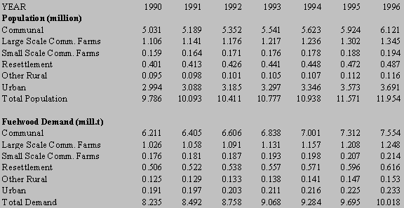
The average annual consumption of fuelwood in non-urban areas ranges from 8.24 million tonnes in 1990 to just over 10 million tons in 1996. By far, the largest component of demand is within the communal areas, which contain approximately 70 percent of the country’s total population. Given the estimating methods used, fuelwood consumption mirrors population growth.

The amount of fuelwood derived from agricultural field clearance must be subtracted from the gross depletion figures since the timber felling arises from shifting land-use rather than simply harvesting trees for energy. The fuelwood is a by-product. Based on Atwell et al 1989, and discussions with Forestry Commission staff, we assume that for fuelwood from both urban and rural areas, 50 percent is derived from field clearance.

The amount of fuelwood collected as dry wood must also be subtracted since it does not represent a reduction in standing timber stocks. For urban areas this will be presumed to be zero, based on Campbell and Mangono (1995) which states that most urban fuelwood is cut from indigenous trees. In rural areas, the percentage of households using deadwood for household cooking ranges from 91 percent in resettlement areas (where there is a lot of wood) to 73 percent in communal areas (baseline survey quoted in Campbell and Mangono 1995). This case study uses a figure of 75 percent to carry out the adjustments (Table 5).

The residual is fuelwood cut directly from the standing woodlands and thus contributing to deforestation. From the calculations, this volume amounts to 1.395 million tonnes in 1996.

Table 5 - Total woodland loss after adjusting for dry wood and land clearance, 1990 – 1996.

The area of indigenous woodland in Zimbabwe has shown a continuous decline in the past decade (Table 6). Between 1985 and 1996 the woodlands of Zimbabwe were depleted at an average rate of 2.01 percent per annum. Overall, biomass depletion has been taking place at a uniform rate of 30.1 million tonnes per annum between 1985 and 1996. The depletion rate was greatest in the bushland category (4.14 percent per year). The expansion in the wooded grassland (7.23 percent per year) appears rather high and cannot be easily explained. These figures must be tempered by the knowledge that Forestry Commission’s inventory, growth and yield data for indigenous forests are not well developed. Until recently, the emphasis on forest mensuration has been on managed commercial plantations of exotic pines, which underpin a growing forest industry. It is hoped that in time, more comprehensive and accurate growth and yield data, based on permanent sample plots and remote sensing will emerge from an expanded inventory programme presently being implemented.

The next step is to estimate the net annual increment of the forest after allowing for losses from harvesting for fuelwood (Table 7). The mean annual increment (mai) is the average annual increase in forest stock volume comprising many individual stands and is measured by dividing the cumulative stand volume by the age of the stand (Husch, Miller and Beers, 1972). The mai basically represents forest growth. Mean annual increments were derived from discussions with the Forestry Commission where mai was estimated as 2.23 percent of the total accessible growing stock volume. This approach leaves much to be desired from a mensuration point of view, but it is the best that the Forestry Commission could offer at this time.

Table 6 - Forest cover type changes between 1985 and 1996.

Not all of the forest increment is directly a vailable for fuelwood harvesting as some is in protected forest areas and national parks. In the absence of more recent data, we use the estimates from a study by Touche Ross (1992) which, found that only 30 percent of the mean annual increment is available. Total growing stock from 1990-1996 is derived by beginning with the 1985 growing stock figure from Table 6 (1499.7 million tonnes) and deducting five years of average losses (30.1 million tonnes x 5). The resulting figure (1349.2 million tonnes) is shown for 1990 in Table 7. Thereafter, total growing stocks are reduced by 30.l million tonnes per annum. The accessible growing stock is then calculated by multiplying the total growing stock figures by 30 percent. The net annual increment is calculated as accessible mai less annual depletions.

Table 7 - Net annual increment estimates (million tonnes), 1990 - 1996

Campbell and Mangono (1995) derived estimates of fuelwood prices for each sector from a survey of fuel prices. The average price of rural fuelwood is estimated to be Z$120 per tonne in 1994 while urban fuelwood is Z$230 per tonne. These are then extended to other years based on changes in the consumer price index published by the Central Statistics Organisation (Table 8). A weighted price, based on volumes used (from Campbell and Mangono, 1995) is presented for all years.

Table 8 - Fuelwood prices (Z$/tonne), 1990 – 1996

For household collection costs of fuelwood, an indirect valuation approach is required since most fuelwood is collected in the forest by the consumer rather than purchased through markets. The following opportunity cost method is used:

The amount of time spent collecting firewood is a function of several variables including population in a given area relative to existing forest stocks, rate of deforestation, existence of eucalyptus plantations and their age structures. In the absence of community woodlots, the time required to collect indigenous fuelwood is likely to increase with rising deforestation. Indeed, discussions with the Forestry Commission suggests that in resettlement and well-wooded communal areas, collection trips for wood are largely within one kilometre (km) of the homestead and less than one hour in duration. Collection in deforested areas on the other hand, may be 200 percent longer in duration for firewood and 50 percent longer for construction wood than in well-wooded areas. The general tendency is to do most firewood collection in the dry season compared to the wet season. A comprehensive survey to derive average collection times for fuelwood throughout the country was beyond the scope of this study. Using previous surveys from Campbell and Mangono (1995), rural households spend an average of 10 hours per week collecting firewood in the dry season and four hours per week in the wet season, presumably because agricultural activities are more time consuming in the latter period. The average time per week thus works out to be seven hours per week, slightly higher than the six hours per week for the 1980’s period implied by estimates in Du Toit et al (1984). This is a crude symptom of increasing scarcity of easily accessible forests for domestic fuelwood. Using an average of seven hours per week collecting time, the total time per year is 364 hours. This rate is assumed to remain constant for the period 1990-1996.

The opportunity cost of labour used in the collection of firewood is the cash income the person (usually women) might otherwise have earned by working as unskilled agricultural labour on a commercial farm or horticultural operation. The minimum wage for casual agricultural labour has risen in nominal terms from $100 per month in 1990 to $503 in 1998. It is perhaps unrealistic to suppose that this minimum wage is the true potential earnings (Crowards 1994). In a study of female wage labour in Zimbabwe, Adams (1991) found a value of Z$52 per month for the 1986/87 period, or 61 percent of the minimum wage. We extend this ratio to the period 1990-1996 under the assumption that casual labour wages remain a constant fraction of the minimum agricultural wage, an assumption also used by Crowards (1994). Another approach is to estimate the value of extra food or cash crops that could have been grown in village gardens with the time required instead to collect fuelwood. This approach has merit but no recent studies were available to review.

To calculate the average time spent collecting fuelwood, the average collection time per year (364 hours per household) is divided by the average consumption of fuelwood per household of 6.01 tonnes (from Frost, 1997). The resulting figure of 60.56 hours is assumed to remain constant throughout the study period. Better estimates, perhaps reflecting increased scarcity of fuelwood could only have been derived if time series data were available from surveys. The hourly casual wage is calculated by dividing the casual monthly wage by 242 hours per month, which reflects on average, a 10-hour working day, six days per week. The cost weighting is the same as used by Crowards (1994) and is similar to that derived in Campbell and Mangono (1995) to reflect the higher cost of urban fuelwood to rural fuelwood. The weighted opportunity costs are found by multiplying the collection costs/tonne by the collection cost figures (Table 9).

Table 9 - Opportunity costs of fuelwood extraction (Z$/tonne), 1990 - 1996

Total resource rents for fuelwood are calculated by multiplying average residual or stumpage values (the difference between weighted fuelwood price and weighted cost) by the total annual depletions (Table 10). Estimated rents have been rising rapidly over the period. The average annual increase in rent values over the six-year period is around 72 percent.

Table 10 - Resource rents for fuelwood depletions (million Z$), 1990 - 1996

To estimate Hotelling Rents, the total rent for depletions in Table 10 must be multiplied by the right-hand side of equation 7. In applying equation 7 to the data, a discount rate of 18 percent is used, which represents an average discount rate during the 1980’s and 1990’s. In addition, some estimate of marginal cost elasticity must be used. No published figures are available which lend themselves directly to this case study, however for the purpose of illustrating the method, a marginal cost elasticity of 0.6 is assumed⁶. This figure is equivalent to the FAO estimate of deforestation in Zimbabwe and is comparable to that used by Vincent (1996) for Malaysia. A plausible hypothesis is that average collection distances and hence opportunity costs have increased by this amount during the study period. Clearly, to apply accurate estimates of marginal cost elasticity would require much richer time series data on opportunity costs of fuelwood collection throughout the country. The Hotelling Rent increases significantly over the study period (Table 11).

Table 11 - Total rent and hotelling rent, 1990 – 1996.

Net investment is calculated as gross fixed capital formation minus depreciation of physical capital and Hotelling Rents. Ideally, figures of physical capital depreciation should be obtained from the system of national accounts. Unfortunately, the Central Statistics Office does not collect such figures and could not provide any data. Thus, indirect estimates are required.

A theoretically elegant method for estimating depreciation in view of data gaps is the Perpetual Inventory Method. The last value for the capital stock was contained in the Industrial Census of Production of 1967/68. Extrapolating from this period to the present is fraught with danger. While results are plausible for the early half of the 1970’s, from the 1980’s, the estimation procedure completely breaks down and yields highly implausible results.

An alternate approach to estimate depreciation is to use a version of the Harrod-Domar equation (equation 8).

A routinely used assumption in macroeconomic analysis is that investment cumulates nicely to generate capital growth. Using this assumption, we can compute due allowance for physical depreciation of the existing capital stock at a (constant) rate d⁷ (equation 9):

The national accounts are still the most convenient source of data to estimate the parameters in equations 8 and 9. However, in the absence of capital stock data, professional intuition and the literature must be drawn upon. The stylised fact from the development economics literature is that (aKX) ought to take a value between 2.5 and 6, with 2.5 being considered too low and 6 being on the high side (Taylor 1990). A figure of 4.0 for Zimbabwe is used based on our understanding of the economy and the literature elsewhere. The value of capital implied by a capital-output ration of 4.0 and resulting depreciation for the 1990-1996 period are estimated in Table 12. The rate of depreciation of physical capital for equation 9 is 0.04, a figure which compares well with a figure of 0.043 often used by the National Economic Planning Commission in Zimbabwe.

Table 12 - Estimates of capital and depreciation for Zimbabwe (million Z$), 1990 – 1996.

Equipped with the previous depreciation estimates, CSO data on gross fixed capital formation (GFCF) and Hotelling Rents, the national accounts of Zimbabwe can then be adjusted (Table 13). Net investment⁸ is calculated as GFCF less depreciation and Hotelling Rents. Net domestic product is calculated as GDP less depreciation and Hotelling Rents for fuelwood depletions.

Table 13 - Net investment and net domestic product for Zimbabwe (million Z$), 1990-1996.

At the macro level, net investment was positive throughout the period, suggesting that the economy did better than Hartwick's Rule. A general conclusion, based only on these data, is that the economy could actually have consumed more per capita and still not jeopardised future growth. This result is very robust for a wide range of capital output and depreciation ratios. However, this finding should be qualified by pointing out that we did not adjust for changes in human capital. Also, looking at this from a macro framework may be misleading. From a disaggregated local perspective with a high rate of depletion, the result may be negative. Other studies, such as Vincent (1996) for Malaysia, also found a positive net investment. In Vincent’s study, net investment was negative in only one year out of the 20 evaluated. More discussion about the quality of the results is in section 5.0.

Another way to interpret the data is to consider the annual average percentage changes in both GDP and NDP. If the percentage change in NDP is less than for GDP, there could be concerns raised about the sustainability of fuelwood harvesting at the macro-level. Estimates of average annual percentage changes in GDP and NDP, and the difference between the two percentage changes are shown in Table 14.

Table 14 - Average annual GDP and NDP growth, 1990 - 1996.

Looking at individual years, there is a mix of results and no consistent trend between the rates of average growth as evidenced by the difference between the two values. In three years, GDP growth is slightly less than for NDP; the situation is reversed for the other three years.

These percentage values can also be averaged over the time period. For GDP growth, the average percentage change is 26.09 percent while for NDP the figure is 26.13 percent. In other words, there is virtually no difference betwee n the two estimates. For all intents and purposes and accounting only for fuelwood depletion out of the forest stock, adjusting the system of national accounts results in a very insignificant transformation to NDP. This result implies that in the narrow context of fuelwood harvesting, the economy did indeed grow in a sustainable manner.