![]()
![]()
![]()
M. Rout
Freshwater Aquaculture Research & Training Centre
Dhauli
Composite fish culture or polyculture of indigenous carps together with the Chinese carp and common carp has been found to result in high production of 9 to 10 tons/ha in a year with a stocking density of 7500 to 10,000 and with inputs of feed, fertilizers, organic mahures, lime etc. The evaluation of causative factors by statistical techniques i.e. ecological conditions, feed utilization, applied and available nutrients etc. will help in optimizing the production process. The lecture has been prepared to identify such functional relationships between the response variable and their causative variables and the procedure to estimate the parameters designated in the equation.
The parameters are estimated from a sample size taken from population. Consider the problem of predicting variable Y from P variable X, X2 … Xp (P > 1). The variable Y is called the dependent variable, while variables X1, X2 … Xp are called independent variables. The model equation expressing the relationship between the dependent and independent variables is given by
Y = f (x1 … xp; β1β2 … βm) + e where
β1, β2 … βm are unknown parameters and e is an error variable representing the error incurred in approximating y by the regression function. If f (x1, … xp; β0, β1 .. βp) = β0 + β1 x1 + … + βpxp, then the multiple linear regression model is
Y = β0 + β1 x1 + β2 x2 + … + βpxp + e
and the polynomial regression model is
Y = β0 + β1 x + β2 x2 + … + βpxP + e.
The least square method is employed to estimate the parameters such that
S = Σ ( Yi - β0 - β1x1i - …βp xpi)2 is a minimum. The sum of squares of deviation ‘S’ is a measure of error incurred in fitting the sample with the model. It has been observed that the higher the number of independent variables, the better is the prediction likely to be.
As an illustration, a simple model can be written
for composite culture experiments as
W = a+f+F
Where ‘a’ is the mean natural production of pond, ‘f’ is the
component of production added to it by fertilizers and ‘F’
is the component added to it by feed. W represents the
expected production. The model of above type can be
expressed as
W1 = a + f+ F + e where ‘W1’ is the observed production and ‘e’ is the departure of the model predicted value ‘W’ and the observation ‘W1’ of production.
Consider for example, the relation between the fertilizers applied and the yield of a fish crop. If by applying 100 kg of NPK to a fish pond weight an increase in yield of 200 kg/ha, it is not necessarily likely that 500 kg of it would give an increase of 1000 kg/ha or that 10 kg of it would give an additional yield of 20 kg/ha. Higher and higher fertilizers or feeds application, production may not linearly related and may touch asymptotically at an ultimate weight.
The natural parameters and other major parameters for achieving production in culture experiments have been summarised in subsequent chapters.
In culture experiments, the estimation of standing crop of fish from time to time is required to adopt a judicious management measures for a higher production au well as a lucrative profit. Inaccessibility of fishes to direct observation in their natural habitat raises problems for the biologists. So a basic understanding of population dynamics, production, yield is essential for monitoring the numerical changes which occur in a population in a course of time.
This is based on drawing a sample of marked and unmarked
fishes from a population with known number of marked
and unknown number of unmarked fishes. The ratio of marked
fish recaptured to the total number of fish caught is assumed
to be equal to the ratio of the total marked fish in the
pond to the total population i.e. 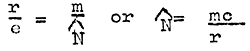
where  = estimated population, m = total no. of marked
fish in the population, c = total no. of fish in the sample,
r = number of marked fish recaptured.
= estimated population, m = total no. of marked
fish in the population, c = total no. of fish in the sample,
r = number of marked fish recaptured.
The estimated population and production of fish are
to be calculated from time to time to study the survival
and the quantum of feed to be required for fish. In a culture
experiment if m = 400, c = 600 and r=100 then the estimated
population 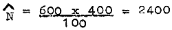
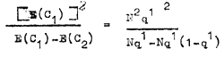
In a short term sequence of identical fishing operations
in a fish pond, the successive catches decline in a
regular manner. If two hauls (C1 & C2) are taken, an
estimate () based on just two trials can be expressed
in the form 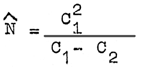
If there are three hauls C1, C2 and C3, each catch
not allowed back to pond, then the estimated population
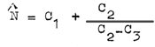
The sequence of expected catches E(C1), E(C2), E(C3) thus follows the pattern Nq1, Nq1 (1-q1), Nq1 (1-q1)2 where q1 is the probability of catch being caught in each trial. The estimate N is based on the catch model
Rate of daily feeding is calculated either as a percentage of the total weight of the standing crop or on the basis of the daily increase in total weight of standing crop. Both the methods are subject to two sources of error. The first is the possible error in estimating the average weight of the population and the second is the error in estimating the number of individuals in a population at one time.
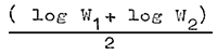
Estimate of standing crop may be made from total amount of daily feed which is expressed as W = IRN or logW = log I + N logR.
W = total weight of standing crop at the end of N intervals of feeding, N = number of ‘T’ intervals during which fish have been fed at rate ‘P’, I = initial weight of fish and R = rate of change in weight during interval T.
Example:- Suppose 40 kg of silvercarp are stocked and fed with supplemental feed, six days weekly with 3 per cent of weight of standing crop for a period of 30 weeks and R = 1.106. Then I = 40, N = 30T, T = 1 week, P = 0.03, Log W = log 40 + 30 log = .106 or log W = 2.91486 or W = 821 kg.
Production is defined as the total elaboration of fish tissue during any time interval. It may be measured in terms of wet weight, dry weight, nitrogen content or energy content. Production studies are based either on measurements of weight or energy contents.
The average size or average weight of fish is calculated when n number of fishes are weighed in one bulk, then the mean is the sum of the values of individuals to the total number of individuals.
Suppose there are n different values x1, x2, x3… xn
which occur respectively f1, f2 … fn times. Then
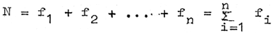 The mean x of the
N values of the variable is given by
The mean x of the
N values of the variable is given by

since the value xi occurs fi times. This is also called as the weighted mean of the different values xi whose weights are their frequenceis fi.
The variance of the weight distribution is estimated
as 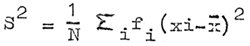 which may be taken as an indication
of the extent to which the values of x are scattered.
which may be taken as an indication
of the extent to which the values of x are scattered.
Production can be estimated for each interval in a well arranged composite culture pond where natural mortality is almost absent except under severely adverse conditions such as depletion of oxygen, disease and poaching.
When the stock size remains constant i.e. no mortality during the period of culture, the production is Nx(W2-W1) where W1s are average weights at start (w1) and end (W2) of the interval.
When there is mortality during the period of culture
and time is not known, the production is given by
N1 ( -W1)+N2 (W2-) where 1, 2 are suffixes for start
and end points of time interval and = antilog
-W1)+N2 (W2-) where 1, 2 are suffixes for start
and end points of time interval and = antilog
The periods in which sudden mortalities are observed and average weight (W) and number (N=N2) is observed immediately after the mortality; production is given by N1 (W-W1) + N2 (W2-W)
Example:- Suppose in a composite culture experiment, the growth and survival of fishes are as follows:
| Time | Number per present | Average weight (g) | |
| Stocking | 1000 | 10 | |
| After one month | 600 | 40 | |
| After sixth month | 600 | 800 | |
| Harvest after 10 months | 500 | 1000 |
Production can be estimated in two ways:
i) General method:
Production = N2 × final weight-N1 × initial weight
= 500 × 1000-1000×10 = 490 kg.
ii) Suggested method:
Production for the 1st
month = N1(-Wo) + N2 (W2-)
= 1000(20-10)+600(40-20) = 22 kg

Production for 2nd to 6th month = 600 (800-40) = 456 kg Production for 7th to 10th month = 500 (1000-800) = 100 kg Total production = 22 + 456 + 100 = 578 kg The difference of (578-490) = 88 kg in production loss is due to overall calculation for estimating production.
An individual fish in a stock increase in size, at the same time, the numbers are reduced from the stock because of mortality. The mass of a whole stock at a given time is determined by the resultant of the forces of growth and of mortality.
In practice, neither growth nor mortality is likely to be exponential for any longer period of time, but those expressions can be used as approximations, being better, the shorter the interval. Any growth curve can be treated in this way if it is divided up in to short segments.
When growth is considered to be exponential, its
instantaneous coefficient G is estimated by
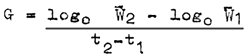 where 1, 2 are the mean weights
of fish at times t1 & t2, respectively.
where 1, 2 are the mean weights
of fish at times t1 & t2, respectively.
Consider Wj(t) be the body weight of an average
species j carp at time t. Then the growth of fish per time
unit  is a model which is also called as an INPUT/
OUTPUT model i.e.
is a model which is also called as an INPUT/
OUTPUT model i.e.  = INPUT-OUTPUT
Example: A fish in culture experiment grew from .1 to 1.5 kg
in unit time, say, a year then the absolute growth is 1.5–0.1
= 1.4 kg per year. Its relative growth or annual growth rate
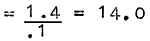 = 14.0 i.e. 1400% per year. The instantaneous rate of
growth is loge
= 14.0 i.e. 1400% per year. The instantaneous rate of
growth is loge 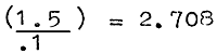
The most useful manner of expressing the decay (decrease) of an age group of fishes through time by means of exponential rates and are expressed as follows:
Nt = No e-zt where ‘No’ is the initial number of fishes at time t = O and ‘Nt’ is the number of remaining fishes at the end of time ‘t’ and ‘z’ being the instantaneous rate of total mortality.
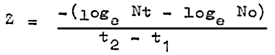
Nt, No are the number of fishes present at times t1 and t2.
The differences G-Z is the net rate of increase in biomass during the time t2-t1. Also Z = M+F where M is the instantaneous rate of natural mortality and F is the instantaneous rate of fishing mortality. When F = O, Z = M which means that total mortality and natural mortality have the same value where there is no fishing. Modelling population decay in culture fishery by an exponential Nt = No e-zt is hardly valid except in the early phase of stocking when sizeable mortalities have been reported due to weak or too small sizes at stocking.
Production may be estimated graphically when data on
growth and survivorship of fish are available over the time
span of interest. In this method, the number of individuals
(N) in the population at successive instants of time are plotted
against the mean weight () of an individual at the same instants.
A hypothetical example from an experimental pond is illustrated in Fig.-1.
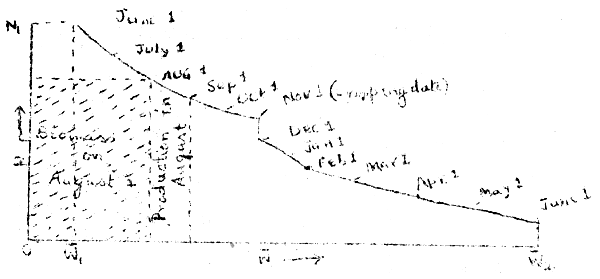
Fig. 1. Seasonal changes in numbers (N) and average
weight () of fish in a pond.
In June 1st, stocking was done and on 1st of every-month sampling was made. The estimate of population number and mean size were collected and put in the graph. Production in August is equal to the shaded area beneath the curve. Biomass on August 1 is shown on the graph. Annual production is the entire area beneath the curve from June 1 to June 1, a year later. Areas can be measured on the graph by using a planimeter. If the curve is plotted on graph paper, areas can be measured by counting squares.
Technique of multivariate data analysis relates to the study of interrelationship between inputs and output. Ecological variables and input variables from an environment which are mostly interrelated can be evaluated. Use of different inputs (independent variables) in ponds may enable us to predict the output (dependent variable). This requires the application of the multiple regression techniques. The more common data interpretation techniques are covered here.
Multiple regression provides an analysis of the relations among two or more predictor variables and a single criterion variable. One result of the analysis is an equation for predicting the criterion score of a subject from its known set of predictor scrores. If Y is the criterion variable, the relationship between Y and the X's is formulated as a lenear model i.e.
Y = ao + b1x1 + b2x2 + … + bm xm + o
or Y = ao + ∑ bi xi = o
where ao is overall mean corresponding to mean levels of xs; bs, are regression coefficients and e the residual “error” term of departure of individual Y values from model.
To illustrate the model in composite culture experiments, we can treat fish growth (or production) Y over a period as criterion or response variable determined by the joint effects of predictor variables such as area of pond (x1), number of fish stocked (x2), fertilizers applied (x3), manures put (x4), feed given (x5). Then the multiple regression equation is Y = a+b1x1+b2x2 + b3x3 + b4x4 + b5x5 + e
It is assumed that this regression equation provides an acceptable approximation to the truo relationship between Y and the x's. In other words, Y is an approximatel linear function of the x's and e measures the discrepancy in that approximation.
In this approach, aquaculture production or growth would be related to various factors in a sequencial fashion, with the sequence being directly related to the explanatory power of the factor. The procedure allows one to observe the partial effect of a factor while at the sametime considering only those factors for which the data suggests a relationship. It is conceivable that after considering four or five of the factors according to their magnitude of correlation, the remaining factors do not add much to the explanation of production or growth.
This method is highly laborious and is generally handled on computer. Statistical software package on stepwise regression is available mostly in FORTRAN language.
Regression analysis by least squares technique implicitly assumes that the predictor variables are uncorrelated with each other. With this assumption in mind, it is usual to interpret a regression coefficient as measuring the change in the response variable when the corresponding predictor variable is increased by one unit and all other predictor variables are held constant.
If there are p variables i.e. 1 response and P-1 predictors then the data sets involve p means, p variances and P(P-1)/2 correlations to interpret and estimate. One way of getting out of this is to search for uncorrelated predictor variables. Since correlation coefficients only sore up the parameters and interpretation problems, we seek to have those which have zero correlations.
Let the regression model stated in terms of original standardized variables be
Y = β1X1 + β2X2 + … + βpXp + V
The above equation may be written in terms of the principal components as Y = α1Z1 + α2Z2 + … + αpZp + V.
The α's and may be obtained by the regression of Y against the principal components Z's or against the original standard variables x's. The principal components regression is used as a means for deleting and analysing the problem of multicollinearity. The final regression estimates are always restated in terms of β's for interpretation.
A suitable computer program for regression analysis by principal components approach is developed. Regression analysis for a set of maximum up to 40 variables including the response variable can be performed.
The interrelationships between two sets of measurements made on the same subject can be studied by canonical correlation method. The canonical correlation is the maximum correlation between linear functions of the two vector variables. That is, each pair of functions is so determined as to maximize the correlation between the new pair of canonical variates, subject to restriction that they may be entirely orthogonal to all previously derived linear combinations.
For example, in composite culture experiment, if there
are production of six species from eight inputs applied to
the pond, then there are 48 correlations between production
and inputs. If there are P1 elements in Z1 and P2 elements
in Z2 and P = P1 + P2 then the square, symetric correlation
matrix R of order P is sub-divided in to 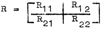 such that R11 contains the inter correlations
among the elements of Z1 and is of order P1, R22 is the inter
correlations among the elements of Z2 and is of order P2.
R12 = R21 contains the cross correlations between elements
of Z1 and Z2 and is of order P1 × P2.
such that R11 contains the inter correlations
among the elements of Z1 and is of order P1, R22 is the inter
correlations among the elements of Z2 and is of order P2.
R12 = R21 contains the cross correlations between elements
of Z1 and Z2 and is of order P1 × P2.
This method is an extension with much more soundness and having the direct property of immediate identification of response correlations with the predictors. Computer software programmes are available for this.
Composite culture of indigenous and exotic species with balanced fish food, judicious fertilization, elimination of accumulated metabolities has shown the practicability of enhancing fish production. But at higher level of manure application and higher rate of feeding, the physico chemical characters change, natural primary productivity affected and large quantities of food remain unutilized. Soil and water characteristics, plankton density, composition in terms of species and size would not remain same and the resultant variations show very high. These systematic causes of variation and the inherent variability can be studied by use of different statistical tests to identify the degree of error variations and corrections needed for achieving the goal within reasonable limit. To estimate the population parameters affecting the growth and production, the sample, functions are to be built by applying proper sampling techniques.
The use of advanced statistical techniques has been significantly increased since the introduction of computers. The agricultural statisticians, economists, soil scientists, fishery biologists are to work with full cooperation by using more sophisticated methods of analysis. In culture experiments, any number of variables limiting to the capacity of the computer, chemical parameters or biological indicators effecting production can be analysed and interpreted. Techniques of linear programming, multivariate least squares analysis, factor and path analysis, D2 statistics are also some of the useful and important methods for analysing data. Multivariate analysis presents no problem when computerisation is done for any number of variables. So greater coordination is needed between the aquaculture researcher and applied statistician for indepth analysis of various problems in aquaculture.
Afifi, A.A. and S.P. Azen (1979).
Statistical Analysis - A Computer Oriented Approach.
Academic Press, New York, 442 P.
Anderson, T.W. (1958)
An Introduction to Multivariate Statistical Analysis
John Wiley & Sons, Canada, 374 P.
Cochran, W and G.M. Cox (1957)
Experimental Designs. John Wiley, New York.
Cooley, W.W. and P.R. Lohnes (1971)
Multivariate Data Analysis. John Wiley, New York, 314 P.
Doshi, S.P. and Ram Kumar (1981).
User's Manual and Fortran Programs for Regression
Analysis. Indian Agricultural Statistics Research
Institute, New Delhi-12, 45P.
Kendall, M.G. (1957)
A Course in Multivariate Analysis.
Charles Griffin & Co., London.
Por Sparre (1984)
A Programme of Bioeconomic modelling on Freshwater
Fish Culture in India. Report. FAO/UNDP/75/031, Rome, 89P
Snedecer, G.W. (1961). Statistical Methods.
Allied Pacific Private Ltd., Bombay, 534 P.
![]()
![]()
![]()