Getting the accounting framework right for forest resources is the easy part. Implementing the framework is considerably more difficult. Implementation raises conceptual issues related to methods for calculating entries in the framework. Once those issues are resolved, one faces the challenge of compiling adequate data for applying the methods. This chapter addresses conceptual issues related to methods, and the next considers the feasibility of implementing the methods as revealed by recent empirical studies.
In the previous chapter, we identified eight basic accounting adjustments related to economic aspects of forests:
To be added to GDP
Final consumption of nonmarket forest products
Final consumption of forest amenities
To be reallocated within GDP
Environmental services of forests
Pollution deposition in forests
To be added to NDP
Net accumulation of timber
Net accumulation of carbon
Net accumulation of forestland
Net accumulation of converted land
Implementing the first four adjustments and the sixth (carbon) is a matter of applying nonmarket valuation techniques. Much experience has been gained with these techniques during the past twenty years. Several book-length treatments are now available (e.g. Boardman et al. 1996, Dixon et al. 1995, Freeman 1993, and Smith 1996), and literally thousands of articles have been written. Reviewing the range of available techniques, and experience with them, is far beyond the scope of this report, and indeed it was not included in the terms of reference for the report.
For these reasons, this chapter will primarily focus on valuation issues related to timber and land. These aspects of forests pertain to two of the major policy issues related to forests, timber depletion and deforestation. They also involve unique economic features of forests, such as long rotation cycles. The studies reviewed in the next chapter indicate that adjustments related to timber are typically the most feasible ones to implement, and usually the largest.
Before discussing timber and land issues, however, we will offer a few observations related to other adjustments. These observations take advantage of information generated by the model in Appendix 1, and they provide background concepts necessary for evaluating the studies in the next chapter.
Nonmarket values
Three of the adjustments in the above list relate to nonmarket impacts on output in other industries: environmental services, pollution deposition, and CO2 sequestration. For example, agriculture and hydropower benefit from the free watershed protection services provided by forests. Similarly, manufacturing benefits from pollution deposited in forests because it does not have to pay to abate the pollution. If it did, its profits and output would be lower. Lastly, climate-sensitive industries benefit from carbon sequestered in forests because sequestration reduces the risk of climate change and its deleterious consequences.
For these entries, the most straightforward valuation method to apply, and the one implied by the model in Appendix 1, is the productivity change method. For environmental services, application of this method involves calculating the following expression:
Area of forest providing environmental service
|
x |
Hypothetical increase in current output of the industry receiving the service if forest area were to increase by one unit |
|
x |
Unit value (price) of output of industry receiving the service. |
The second line gives the marginal product of forests in providing the service; in combination, the second and third lines give the marginal value product of forests as a source of the environmental service. Note that the first line includes only the forest area actually providing the service, not the total forest area. Including total forest area would overstate the value of the service. As discussed in Chapter 2, the estimated amount given by the above expression should be subtracted from value added of the industry receiving the benefits and added to forestry value added.
For pollution deposition, two expressions are possible. The first is similar to the one above:
Amount of pollution deposited in the forest
|
x |
Hypothetical increase in current output of the polluting industry if it were allowed to emit one more unit of pollution |
|
x |
Unit value (price) of output of the polluting industry. |
This is equivalent to:
Amount of pollution deposited in the forest
|
x |
Cost of abating the last (marginal) unit of pollution. |
The second expression is in terms of forest damage:
Amount of pollution deposited in the forest
|
x |
Hypothetical decrease in current growth of timber if the polluting industry were allowed to emit one more unit of pollution |
|
x |
Sum of stumpage and carbon sequestration values of a unit of timber. |
As in the case of environmental services, the calculated amount from either expression should be subtracted from value added in the polluting industry and added to forestry value added.
If pollution is at the optimal level, so that the marginal benefit of abating pollution equals the marginal cost, then the two expressions should yield the same calculated amount. When pollution is above or below the optimal level, however, the two expressions yield different amounts. In this case, which is the usual case in practice, the second expression is preferred, as it measures the forgone benefits provided by forests — the opportunity cost of timber output and carbon sequestration services that society sacrifices — and thus indicates the welfare impact of using forests for pollution disposal.
For carbon sequestration, the expression is more complicated, as the adjustment is to NDP, not GDP:
Net sequestration of carbon in the forest (release minus uptake)
|
x |
Present value of hypothetical future increases in the value of output of climate-sensitive industries if one more ton of carbon were sequestered. |
Note that net sequestration can be either positive or negative. In either case, the product of it and the second term should be added to NDP. Obviously, the most difficult step here is to calculate the second term, which gives the long-run, avoided damages resulting from carbon sequestration in the forest. The most feasible approach is probably to base the value on predictions of economic models of climate change. Nordhaus (1994), for example, estimated a 1995 value of US$5.24 per ton of carbon (at 1989 price levels).
The two entries related to nonmarket consumption require a different valuation approach, as in those cases the economic contribution of forests is not operating through production relationships. For household collection of nonmarket forest products, the model in Appendix 1 implies using the following opportunity cost method to calculate a lower-bound estimate:
Amount of time spent collecting x Opportunity cost of time.
The calculated amount should be added to GDP. Note that this expression does not include the cost of purchased intermediate inputs (e.g., bags, tools, transportation), as GDP is net of purchases of intermediate inputs (double-counting would occur if they were included in the formula above). If such inputs are made by households rather than purchased, however, then the time spent making them should be included. Nor does the expression include forest fees paid to the government or other forest landowners, as those fees are (or should be) already included in GDP.
This last point, however, gets at the reason why the expression given above yields a lower-bound rather than a complete estimate. In many instances, particularly in developing countries, forest ownership rights are not well-defined or enforced. Consequently, collectors of nonmarket forest products often do not have to pay for the use of forest resources. In a situation of complete open-access, one expects that this will cause forest rent to be completely dissipated: households will collect nonmarket products up to the point where the perceived value of the last unit collected just equals the opportunity cost of labor used to collect it. That is, they will ignore impacts on forest productivity, for example whether collecting less in the current period would make more available in future periods. In this situation, the (suboptimal) value of collection simply equals the opportunity cost of labor involved. If, however, customary rights prevent the complete dissipation of forest rent, then the full value of collection of nonmarket forest products is given by the sum of forest rent and the opportunity cost of labor.
Valuation of nonmarket forest products is easiest when some portion of the amount collected is sold in markets. Then, collection can be valued simply by multiplying the amount collected times the market price, as long as the products consumed and the products sold do not differ appreciably. Similarly, collection can be valued by the price of a substitute product when the degree of substitution is high (and by more advanced valuation methods when it is not).
The last nonmarket value, final consumption of forest amenities, is the most difficult to value. We have defined this as a non-use value: its production does not require any expenditure on market goods or any input of labor or other factors. An example would be the existence value of biodiversity. To estimate such a value, there appears to be little choice but to apply the contingent-valuation method, which involves asking a sample of individuals to state their willingness-to-pay to protect the nonmarket benefit or their willingness-to-accept to forgo it. When consumption of amenities involves the purchase of other goods, for example when one must drive to a park and pay an entrance fee to enjoy the amenities in the park, then other methods, such as the travel-cost and hedonic-pricing methods, can be applied.
Timber values
Understanding the relationship between asset value and direct methods for estimating net accumulation is easier in the case of a nonrenewable resource than in the case of renewable resources like forests. For that reason, in this section we first discuss the nonrenewable case. Then, we examine how the introduction of renew ability (timber growth) and the typically long time period between regeneration and harvest complicates matters in the case of forests.
Asset value and net accumulation for a nonrenewable resource
The asset value of a natural resource, whether nonrenewable or renewable, equals the discounted sum of the net returns (resource rents) it generates over time. For a nonrenewable resource, asset value at time t is therefore given by
where the sum is evaluated over the interval s = t, …, T. i is the discrete discount rate, p is the price of one unit of the extracted resource (assumed to be constant over time), q(s) is the quantity extracted in period s, C(q(s)) is the total extraction cost, and T is the terminal time (the period when the resource is exhausted). The difference, pq(s) - C(q(s)), is current resource rent. By separating out resource rent in period t, which is not discounted, from the discounted sum, we can equivalently express asset value as
V(t+1) is simply asset value one period later, in period t+1.
Net accumulation equals asset value at the end of a period (i.e., at the beginning of the next period) minus asset value at the beginning of the period:
Substituting the second expression for Vt into this expression, we obtain
This is the fundamental equation of asset equilibrium (Hartwick and Hageman 1993). It indicates that net accumulation is the difference between two opposing forces: the shifting of the discounted stream of future rents toward the present, which increases asset value (net accumulation tends toward a positive value), and the realization of current resource rent, which decreases asset value (net accumulation tends toward a negative value). Hence, net accumulation is not equal to the negative of current resource rent, which most applied studies have assumed to be the case. Under the assumptions we have made, net accumulation is indeed negative (the latter force outweighs the former), but it is smaller in absolute value than current resource rent.
In Appendix 2, we demonstrate that if the assumptions underlying the simple model presented above hold — in particular, if the resource is extracted optimally (to maximize the discounted sum of rents), and if prices, the extraction cost schedule, and the discount rate are constant over time — then one can estimate net accumulation directly, without needing to calculate the present value of future flows of rents. Two basic approaches, which in theory should yield equivalent results, are available. The first is commonly called the net price method. According to this method, one multiplies the marginal net price of the resource (price minus marginal cost) times the negative of the amount extracted:
The use of marginal net price instead of average net price might appear to be a minor detail, but in fact it is crucial: if one uses average net price, then one is calculating the negative of total resource rent, which as noted above overstates net accumulation.
Data on marginal costs are typically hard to obtain or unavailable altogether. If, however, data are available on average cost and the elasticity of the marginal cost curve (percentage change in marginal cost per 1-percent change in quantity extracted), then one can apply the net price method by using the expression,
where C(q(t))/q(t) is average extraction cost and ß is the elasticity of the marginal cost curve.
The second direct estimation approach also makes use of the marginal cost elasticity. Under this approach, which we refer to as the El Serafy method, one multiplies the negative of total resource rent times a conversion factor involving the discount rate, the number of years until the resource is exhausted (T-t), and the elasticity (see Vincent 1997):
This is a generalized version of the original El Serafy method (El Serafy 1989), which implicitly assumes that ß = ∞ and thus reduces to
Note that this simplified version of the formula yields accurate estimates of net accumulation only if the marginal cost elasticity does indeed equal infinity. This is highly unlikely in practice, so one is better off using the version including the marginal cost elasticity. Some authors have referred to the El Serafy method as the user-cost method, but we will eschew this terminology as it creates confusion with the standard meaning of "user cost" among resource economists.13
Net accumulation of timber: the net depletion method
As we will see in the next chapter, both the net price and El Serafy methods have been applied to timber resources. The former has been the most popular, and in applications to timber it is perhaps best described as the net depletion method. Typically, one calculates the net depletion of the timber stock by subtracting growth (and other additions) from harvest (and other subtractions). Then, one multiplies the negative of the resulting amount times net price:
g(S(t)) is growth of the timber stock in period t. This expression assumes that the cost function is nonlinear, and so it includes marginal net price. Alternatively, if costs are linear (C(q(t)) = cq(t)), then one can apply
This expression is really just a special case of the preceding one: when the cost function is linear, marginal cost (C'(q(t)) equals average cost (c).
Although the net depletion method might seem to be a reasonable generalization of the net price method, it does not yield accurate estimates of net accumulation of timber. The reasons are easy to see if one separates the expression into its two components, for harvest and for growth. We begin by disaggregating the forest by age class: AT hectares of mature forest are harvested in a given period, and At hectares of immature forests of ages t = 1, …, T-1 are left to grow. Note that t now refers to age of the forest, not year, and that there are several age classes of immature forests, not just one. Assuming that: (i) forests are even-aged (all trees in a stand are the same age), (ii) all standing timber is harvested at the optimal rotation age T, with no intervening production (e.g., from thinnings), and (iii) q(T) is the standing timber volume per hectare in mature forests, then total harvest equals ATq(T). Similarly, timber growth for forests in age class t equals Atq'(t), where q'(t) is the derivative of the timber volume function.
Net accumulation for a forest disaggregated by age class equals
where DH(T) and DH(t) represent per-hectare net accumulation values of mature and immature forests, respectively. The sum in the second term is evaluated over the interval t =1, …, T-1: "immature forests" is not a single category, but rather a shorthand phrase for all forests that are left to grow during the current period rather than being harvested.
On a per-hectare basis, and using our new notation, the net depletion method amounts to applying the following expressions to mature and immature forests:
Net depletion method

The first expression states that the change in value of one hectare of mature forest equals the product of marginal net price and the negative of volume harvested. This would seem to be analogous to the expression for nonrenewable resources. Of course, renewable and nonrenewable resources differ due to the fact that the former can grow back. For this reason, one should suspect that this expression is incorrect. The change in value of a hectare of mature forest should also reflect the value of future harvests, assuming that the land remains under forest cover.
Grounds for suspicion about the expression for immature forests are even more obvious. The second expression states that the change in value of one hectare of immature forest equals the product of marginal net price and the volume of current growth. Yet, the timber is not yet mature, so it is surprising that it is being valued by the same factor (marginal net price) applied to mature timber. One should expect that the number of years until harvest (the degree of immaturity) somehow needs to be factored in.
Net accumulation of timber: correct methods
In Appendix 2, we demonstrate that these concerns about the net depletion method are valid. We derive two alternative, but equivalent, sets of expressions for calculating the net accumulation of timber. These methods can also be applied to any other forest product produced at intervals of more than one year (i.e., requiring more than a year between regeneration and harvest).
The first set, which is the correct version of the net price method when applied to timber and can therefore be referred to as the net price variation, is
Net price variation


Two differences relative to the net depletion method are immediately obvious. First, for mature forests, the net depletion method includes the harvest volume at the optimal rotation age, while the correct expression (the first one above) includes growth at the optimal rotation age. Second, for immature forests, the net depletion method includes current growth, while the correct expression (the second one above) includes growth at the optimal rotation age. Hence, to calculate net accumulation of timber using the net price variation, one requires data on: the marginal net price of harvested timber (which equals the average net price if the cost function is linear), the growth rate per hectare at the optimal rotation age (the current annual increment, not the mean annual increment), the age of the forest, the optimal rotation age, and the discount rate.
The second set of expressions, which is identical to the first set and is the correct version of the El Serafy method when applied to timber (hence, we dub it the El Serafy variation), is
El Serafy variation

Two obvious differences compared to El Serafy’s method for nonrenewable resources are that the marginal cost elasticity does not appear and that the discounting terms are more complex (note that they differ for mature and immature forests). These differences are related: the complexity of the discounting term reflects not only the delay between regeneration and harvest, but also the economic condition for selecting the optimal rotation age. In the case of El Serafy’s method for nonrenewable resources, the marginal cost elasticity enters for a reason analogous to the latter, i.e. Hotelling’s rule. Although one does not need data on growth increment to apply these expressions, one does need, in addition to data on resource rent (stumpage value) per hectare of harvested forest, data on age of the forest, the optimal rotation age, and the discount rate.
Note that the volume of growth in the first set of expressions (q'(T )) and the harvest volume in the second set (q(T )) both pertain to merchantable volumes: timber in trees of commercial species, net of defect. Calculating net accumulation on the basis of net growth of wood in trees of all species (in the case of the first set of expressions) or gross harvest volume (in the case of the second) would generate upwardly biased estimates. It is also possible to show (see Vincent 1997) that no downward adjustment to net accumulation needs to be made for normal (strictly speaking, optimal) levels of logging damage.
Both sets of expressions are considerably more complex than their counterparts for nonrenewable resources, and more complex than the expression for the net depletion method. If the values they generate are not appreciably different from the incorrect values generated by the net depletion method, then applying them might not be worth the extra difficulty. In Appendix 2, we demonstrate that the net depletion method tends to overstate the decrease in value when mature forests are harvested, with the degree of error depending on the linearity of the cost function. It also overstates the increase in value of immature forests due to growth, except in very young forests when the volume-age relationship has a logistic (S-shaped) form. Since the biases are in opposite directions (negative for mature forests, positive for immature forests), they are to some extent offsetting at the level of the forest estate, which includes a mix of mature and immature forests.
The net impact of the two biases therefore depends on the relative areas of forests in different age classes. If the forest estate consists primarily of mature and very immature forests, which is more likely to be true in developing countries, then the net depletion method will tend to produce downwardly biased estimates of net accumulation of timber in the forest estate. The asset value of the forest estate will appear to be falling more rapidly than it actually is. In contrast, if the forest estate consists primarily of well-established immature forests, which is more likely to be true in developed countries, then the net depletion method will tend to produce upwardly biased estimates of net accumulation. The value of the forest estate will appear to be rising more rapidly than it is.
Only in the case of the forester’s ideal, or "normal" forest, which has equal areas in each age class, does the net depletion method yield an unbiased estimate of net accumulation. In that special case, net accumulation trivially equals zero, because the age-class structure of the forest is stationary from one period to the next. Unfortunately for the net depletion method, "normal" forests are much more common in forestry textbooks than in the real world. Even in the unlikely event that some country’s forest estate is indeed "normal," there is no need to apply the net depletion method or any other method for that matter, as one knows a priori that net accumulation equals zero.
An empirical comparison of the net depletion method to the correct methods
Table 4 compares the various methods for the same forest at different ages. The data are drawn from dipterocarp forests in Malaysia. The relationship between standing volume per hectare (net of defect) and age is given by
which has a logistic shape. Log price (p) is RM115/m3 (1978 price levels), where 1 RM (ringgit Malaysia) ≡ US$0.40. The logging cost function is linear, with c = RM45/m3, and the discount rate is 4 percent (real terms). Under these assumptions, the optimal rotation age (T) is 33 years. The harvest is 37.9 m3/ha, and the resource rent associated with that harvest volume is RM2,650/ha, since the marginal (= average) net price is RM70/m3.
The column headed "Present value" shows net accumulation calculated as the difference between present values. For t = 33, the formula used is V(1)-V(T). As expected, net accumulation is positive (asset value is rising) during the years leading up to harvest, with its level increasing. The columns headed "El Serafy variation" and "Net price variation" show net accumulation calculated using the correct versions of those methods for timber resources. The estimates are exactly the same as those in the "Present value" column. This simply reflects the fact that the El Serafy and net price variations are derived from the difference between present values (see Appendix 2).
The final column shows estimates calculated from the net depletion method. As expected, the estimates differ from those in the previous three columns, especially for older immature forests. Given the logistic volume-age relationship, the net depletion method understates the increase in value of very young forests (up to age 13), but beyond that point it overstates it. It overstates the decrease in value of the mature forest by 1.5 percent, which is small both in absolute terms and relative to the discrepancies for the immature forest.
A couple of simple examples illustrate the potential magnitude of error associated with the net depletion method. If 90 percent of a country’s forest estate is mature and 10 percent is immature (say, age 10 years), then the correct estimate of net accumulation on the average hectare is -RM2,343:
= (0.9 x -RM2,610) + (0.1 x RM59).
In contrast, the net depletion method predicts -RM2,383:
= (0.9 x -RM2,650) + (0.1 x RM24),
which overstates the actual loss in value by only a tiny amount, 1.7 percent. If all the forest estate is of medium age (e.g., age = 17 years), however, then the net depletion method overstates the actual gain in value by 27 percent (RM99 per hectare vs. a true value of RM78 per hectare).
Perhaps the most interesting example is the following. Suppose that 5 percent of the forest estate is of age 33 years and 95 percent of age 24 years. With this age class structure, timber growth exactly equals harvest. Hence, the net depletion method yields a value of zero.14 The actual weighted-average net accumulation is -RM33 per hectare, however. So, net accumulation does not necessarily equal zero when growth equals harvest. It does so only when there are equal areas in all age classes.
Net accumulation in uneven-aged forests
The net price and El Serafy variations presented above were derived for even-aged forests. These methods can also be applied to uneven-aged forests, as long as harvests are approximately the same each time the forest is harvested. For example, suppose a forest contains three age classes, with the rotation age (chronological age of mature trees at harvest) being 60 years. Then, the forest is harvested every 20 years. This is the cutting cycle. In the expressions for the net price and El Serafy variations, T, the optimal rotation age (60 years), should be replaced by the cutting cycle (20 years) whenever it appears in association with the discount rate (e.g., in the term (1+i)1-T). q(T) still represents the amount of timber harvested per hectare, but this is now less than the standing volume, since some of the standing volume is in immature age classes. Similarly, q'(T) now represents only growth of mature timber. t-T still represents the negative of the number of years until the next harvest, though T is, as noted above, now the cutting cycle instead of the optimal rotation, and t is the number of years since the most recent harvest, not the chronological age of trees.
Asset values of timber
Expressions presented in the preceding sections can be used to make timber-related adjustments to not only the current accounts but also the asset accounts. We have shown how to decompose net accumulation into reductions in asset value due to harvesting of mature forests (on a hectare basis, DH (T )) and increases due to timber growth in immature forests (DH (t )). Incorporating other types of reductions, such as losses due to pests or forest fires, involves straightforward applications of the same valuation principles. For example, fire loss of a hectare of forest of age t changes an asset with a value of VH (t) to one with a value of VH (0). Hence, net accumulation in both the current and asset accounts should include an extra amount, equal to VH(0) - VH (t).
These points suggest the following structure for the accumulation accounts for timber:
|
Net price variation |
El Serafy variation |
|
|
Additions |
||
| Future harvests in immature forests |
|
|
| Future harvests in mature forests |
|
|
|
Subtractions |
||
| Timber harvest |
|
|
| Catastrophic losses |
|
|
We have assumed that the cost function is linear and thus use p - c (average stumpage value) to represent marginal net price. Area variables with an asterisk (i.e., At*, AT*) denote areas suffering from catastrophic losses (fire, pest outbreaks, etc).
For the balance sheets, we need asset values, VH(T) and VH(t). We emphasize that the asset value of the timber stock, ATVH(T) + ∑ AtVH(t), is not equal to the simple product of standing timber volume times net price, even when average and marginal net prices are the same. Assuming that the logging cost function is linear, the asset value of one hectare of mature forest is (see Appendix 2)
The discounting term causes this to be larger than the simple product, (p - c) q(T). The magnitude of the error in using the latter instead of the former is greater for lower discount rates and shorter rotations. For example, the simple product understates the actual asset value of the mature forest by just 0.3 percent when the discount rate is 10 percent and the rotation age 60 years, but by 45 percent when the discount rate is 4 percent and the rotation age is 30 years.
For one hectare of immature forest, actual asset value is:
This is larger than the simple product, (p - c) q(t), because
(1+i)t-T q(T) alone is larger than q(t), because timber growth exceeds the discount rate up to T (otherwise, the forest would be harvested at an even earlier age). Division by the term in brackets makes the right-hand side even larger than the left-hand side.
In sum, the asset value of the forest for timber production is greater than the value predicted by the simple product of net price times standing volume. The simple product understates the actual asset value by an even greater amount if one excludes the timber volume in immature forests, which one might be tempted to do considering that trees in those forests might, at the current moment, be too small to have any commercial value.
Holding gains/losses
In deriving both sets of correct methods for estimating net accumulation, we assumed that log prices and the marginal cost function are constant over time. In reality, both prices and costs fluctuate. Vincent, Panayotou, and Hartwick (1997) have demonstrated how to calculate holding gains/losses for nonrenewable resources directly (that is, without calculating the change in present value). The expression they derived is (not surprisingly) a discounted sum involving future price changes and extraction levels.
Price changes create holding gains/losses in the case of timber resources as well. To our knowledge, however, no one has yet derived a direct expression for calculating them. This is not necessarily cause for concern. Given the long time periods involved in timber production, holding gains/losses are not a serious concern if they are ephemeral, i.e. if prices (specifically, net prices) show no persistent trend over time. If this is the case, then a practical solution is to use a moving average of net prices to remove the effects of more extreme transitory fluctuations.
If, on the other hand, net prices show a trend that is expected to continue for one or more rotations, the effect on net accumulation estimates can be roughly approximated by reducing the discount rate. For example, if the discount rate is 10 percent and net prices are rising at 2 percent, one can calculate net accumulation by using a discount rate of 8 percent. Although this will not yield perfectly precise estimates, in most cases it should yield better estimates than ignoring the trends in net prices altogether. It has the added, and not inconsiderable, virtue of being easy to do.
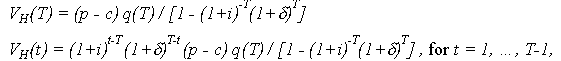
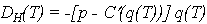
More exactly, when the holding gain/loss is due to a perpetually rising net price that is rising at a constant percentage rate, the asset value of one hectare of forest is given by
where (p - c) is current net price (stumpage value) and δ is the annual percentage increase in net price. Note that setting δ = 0 yields the expression for asset values given in Chapter 3. Net accumulation inclusive of holding gains/losses is now given by
These differ from the expressions given earlier in this chapter, DH(T) and DH(t), which assumed constant net price.
We can use those earlier expressions, however, to isolate holding gains/losses. For a mature forest, the holding gain/loss is given by the difference, DH(T) - DH(T). This just equals zero if δ = 0. The expression for immature forests is analogous. To include the resulting estimates of holding gains/losses in the proposed structure for timber accumulation accounts given above without double-counting, one should calculate other entries in the accounts (i.e., additions due timber growth in mature and immature forests, subtractions due to timber harvest, etc.) under an assumption of constant net prices.
If the gains/losses do not derive from a constant, perpetual percentage increase in net price, the formulation will necessarily be more complex. However, it will always have the general form, holding gains/losses equal actual net accumulation minus hypothetical net accumulation assuming constant net price.
Deforestation
In the notation of the previous section, the asset value of one hectare of forestland for timber production is VH(t) for a forest of age t. If timber is the only benefit provided by forests, then the reduction in asset value due to deforestation is given by the product of area deforested and per-hectare asset value:
If all commercial timber is felled and sold before deforestation occurs, then the second term is the asset value of bare-land, VH(0). In that case, the only loss of timber production is from future rotations, not from the current standing volume. As mentioned in Chapter 2, we recommend including deforestation-induced losses in current standing volume in the net accumulation of timber, not in the net accumulation of forestland.
More generally, of course, forests provide nontimber benefits as well as timber. The decrease in asset value due to deforestation then equals the sum of decreases related to both timber and nontimber benefits. If nontimber benefits are, like timber, provided on a harvest cycle spanning more than one year from regeneration to harvest, then the expression for VH(t) given in the previous section can be applied to calculate their contribution to the value of deforested land. If instead they are provided at a constant annual value per hectare, regardless of the forest’s age, then the loss in value of nontimber benefits due to deforestation is given by the annuity value,
- Area deforested x Annual per-hectare value of nontimber benefits / i .
This expression should be calculated for the full range of nontimber benefits, even those that do not affect the overall level of GDP or NDP: nontimber forest products, forest amenities, environmental services, and carbon sequestration.
If the annual value is not constant—for example, if it rises with the age of the forest—then one needs to perform more complex calculations. If VNH(t) is the annual per-hectare value of nontimber benefits provided by a forest of age t, then the correct expression is:
where s in the first summation (which denotes nontimber values during the remainder of the current rotation) is evaluated from t to T and in the second (which denotes nontimber values during future rotations) is evaluated from 1 to T.
Asset accounts must also include the net accumulation of converted (developed) land. Calculation of this entry depends, of course, on the nature of the use. If the land yields a constant annual per-hectare flow of rent (e.g., annual crop agriculture), then the simple annuity formula applies.
Although the value of developed land is necessarily at least as great as the value of forestland under perfectly efficient markets, with the difference given by land clearing costs (Chapter 2 and Appendix 1), the ubiquity of imperfections in forestland markets due to incomplete property rights and the presence of nonmarket values indicates that one should not automatically set the value of forestland equal to the value of converted land in its new use minus land conversion costs. If one has no choice but to use this formula, then one should be sure to use the value of developed land that actually competes with forestland. For example, if deforestation is occurring in the uplands, one should use the value of agricultural land in the uplands, not an average value, which implicitly includes the value of agriculture in more fertile lowlands.
In Appendices 5 and 6, we provide further analysis of the relative values of forested and converted land.