![]()
![]()
![]()
IGBP Carbon Working Group: Pep Canadell, Kathy Hibbard, Berrien Moore III and Will Steffen.
Abstract
International carbon activities are partitioned into policy, research, observation, and observation platforms. The policy arena is largely delegated through the United Nations Framework Convention on Climate Change (UNFCCC) and the Kyoto Protocol (KP). Global environmental change programmes key to carbon research include the International Geosphere/Biosphere Programme (IGBP), World Climate Research Programme (WCRP), the International Human Dimensions Programme (IHDP), as well as national and regional programmes (USGCRP, CarboEurope, etc.). International assessments of global carbon and climate change issues is relegated to the Intergovernmental Panel on Climate Change (IPCC).
Carbon has been adopted as a theme by the Integrated Global Observing Strategy (IGOS), an initiative of CEOS (Committee on Earth Observing Satellites, representing the major space agencies around the world) as well as the three major global observational programmes, GCOS (Global Climate Observing System), GTOS (Global Terrestrial Observing System) and GOOS (Global Ocean Observing System). In addition, other groups, such as IGBP and WCRP have joined the IGOS group as partners (the IGOS-P consortium - the ‘P’ standing for Partnership).
Through their joint sponsorship of the Terrestrial Observation Panel for Climate (TOPC), GTOS and GCOS have been assigned the lead role in developing the carbon observation theme within IGOS-P. In the realm of the international global environmental change research programmes, IGBP has the lead role in work on the global carbon cycle. Thus, GTOS/GCOS and IGBP have developed a partnership to develop an integrated system for terrestrial carbon monitoring and observation.
The overall goal of the Terrestrial Carbon Observation (TCO) theme is to define observation requirements for an accurate estimation of the distribution of terrestrial carbon sources and sinks of the world with high spatial and temporal resolution. To define the optimal system to achieve this goal requires strong scientific input, both from modelling studies and from ground-based process studies. The GTOS/GCOS-IGBP partnership is designed to build the scientific research-observation community linkages in the most effective and efficient way possible. The workplan outlined for 2000 aims to make use of planned GTOS/GCOS and IGBP meetings in a collaborative way to achieve both observation design (GTOS/GCOS) as well as contributing to an internationally coherent carbon framework focused on research planning and synthesis (IGBP) objectives.
As part of the IGBP synthesis/restructure project, begun in early 1998, it was recognized that IGBP needed to more proactively coordinate the various aspects of carbon research being undertaken in the programme, and the IGBP Carbon Working Group (CWG) was formed. The overall objectives for the IGBP CWG are:
To develop an International Framework for Carbon Cycle Research;
To facilitate and coordinate research, as appropriate, under this Framework, and
To synthesize, at periodic intervals, our latest understanding of the global carbon cycle.
The focus of the work of the CWG has been on the biophysical aspects of the carbon cycle, in keeping with IGBP’s emphasis on biogeochemical cycling. However, there are important aspects of research on the carbon cycle which go beyond IGBP’s remit. Examples include the effects of climate variability on carbon uptake or release (joint WCRP-IGBP issue) and the institutional challenges associated with management of components of the carbon cycle (IHDP issue). Thus, the Chair of the SC-IGBP presented on 13 March 2000 to the Joint Scientific Committee of the World Climate Research Programme (JSC-WCRP) the concept of working together to define an International Framework on Carbon Cycle Research. The JSC-WCRP agreed to this cooperation. In late March 2000, the Chair of the SC-IGBP also presented to the Scientific Committee of the International Human Dimensions Programme (SC-IHDP) an invitation to join with the IGBP and the WCRP in this common activity. It is, thus, that the CWG of the IGBP will become part of a larger consortium based on interaction with WCRP and IHDP, and research on the global carbon cycle will become an inter-programme crosscutting activity. In addition, the IGBP and IPCC have collaborated on schedules and planned activities. The IGBP is aiming to establish a similar relationship with TOPC (Terrestrial Observing Panel on Climate). A summary of the past and current activities and products of the IGBP Carbon Working Group is given below.
Activities of the IGBP Carbon Working Group undertaken in 1998 and 1999
|
Activity |
Time |
Venue |
Product |
|
Terrestrial C Cycle and Kyoto Protocol: Workshop - IGBP Terrestrial C Working Group |
Apr 1998 |
Stockhom, SE |
Science paper (Science 280: 1393-1394 (1998)) |
|
Scoping Meeting: IGBP Carbon Working Group |
Mar 1999 |
Isle sur la Sorge, France |
Overview paper on the global carbon cycle |
|
IGBP Congress: Synthesis Working Session |
May 1999 |
Shonan Village, Japan |
Refinement of Overview |
|
Focused workshop: nutrient constraints on carbon cycle |
Oct 1999 |
Stockholm, SE |
Science paper (submitted Dec 99) |
The IGBP carbon workplan for 2000 is aimed strongly towards completing the synthesis project on the global carbon cycle and on further developing the framework for an international collaborative research on carbon. A number of key activities, which will be carried out in collaboration with the IPCC and the TCO initiative, amongst others, are set out in the table below. The most important of these activities are two major meetings, in May and October. The first is aimed at producing an integrated, DRAFT International Framework for Terrestrial Carbon Cycle research and observation for the next decade as well as an initial draft of the state of terrestrial carbon research. The second meeting is focused on vetting a series of linked articles on the carbon cycle (possibly submitted to Nature) and completing a DRAFT International Framework on the Global Carbon Cycle research. The IGBP, in collaboration with WCRP and IGOS-P have developed the following key activities planned for 2000:
Key Activities of the IGBP Carbon Working Group planned for 2000
|
Activity |
Time |
Venue |
Product |
|
TCO Preliminary Planning Meeting (GTOS/GCOS lead) |
8-10 Feb |
Ottawa, Canada |
‘Strawman’ framework for terrestrial C observations |
|
Workshop on Terrestrial C Research and Observations (joint GTOS/GCOS-IGBP) |
22-26 May |
Portugal |
DRAFT Framework for int’l, integrated approach to terrestrial C research and observations |
|
Global C Cycle Synthesis Workshop (IGBP) |
16-20 Oct |
University of New Hampshire, USA |
A series of linked articles on the carbon cycle and a DRAFT International Framework for Global Carbon Cycle Research |
The objectives for the TCO Planning meeting are to:
Review and synthesize existing plans and specifications for terrestrial carbon observation schemes;
Prepare a ‘straw-man’ framework based on the above;
Recommend strategies for flexibility in future terrestrial observing systems with respect to technologies and in situ observations.
The primary objectives for the May terrestrial meeting where paraticipants will include members from the global modelling community, process studies, and observing systems are:
To develop an INTEGRATED international framework for terrestrial carbon cycle research and observations through to the next decade (and beyond);
To produce a detailed plan for an integrated approach to terrestrial carbon observations: special emphasis on the spatial and temporal distribution of carbon sources and sinks (GTOS objective);
Produce a detailed framework for international terrestrial carbon cycle research including: process studies, modelling, and observation strategies (IGBP objective).
The October meeting will largely be aimed at completing a DRAFT International Framework for Global Carboy Cycle Research and will be built around a number of key scientific questions about the global carbon cycle that are best addressed through international collaboration. The Framework will place a strong emphasis on integration across a number of dimensions and themes:
1) Across oceanic, atmospheric, and terrestrial components of the carbon cycle;
2) Between process studies, experiments, observations, modelling and palaeo studies, and
3) Amongst national, regional, and international contributing projects and programmes.
Finally, as mentioned a second objective of the Durham Workshop is to review and finalize a set of linked articles on the carbon cycle establishing clearly our understanding of the current state of global carbon cycle research and the clear next steps. These articles will establish a firm foundation for the DRAFT International Framework for Global Carbon Cycle Research.
J. Cihlar and S. Brown
1. GENERAL
The purpose of the IPCC guidelines is to support the implementation of the UN Framework Convention on Climate Change (UNFCCC). As part of the Convention, countries agreed to report on the emissions of greenhouse gases, and the Intergovernmnetal Panel for Climate Change (IPCC) subsequently prepared a set of guidelines for such reports. The purpose of the guidelines is to faciliate estimation and reporting on national inventories of anthropogenic GHG emissions and removals, in a consistent format. The Guidelines are concered with emissions and removals that are a direct result of human activities or of natural processes that have been affected by human activities; within national territories (there are four exceptions, such as the decay of all wood products which are assumed to take place in producing country within one year of harvest). Any emissions or removals fitting the above description may be included if they can be clearly documented and quantified. The emissions are reported annually but the temporal resolution is to be compatible with data quality or availability. For example, a 3-year average is preferred for agriculture, and the resolution could be five or more years in forestry because of typical inventory cycles. In addition to annual reports, a complete inventory is also requested for 1990.
Two important methodological assumptions have been made for land use change and forestry: (a) flux is assumed to be equal to change in stocks, and emission factors for non-CO2 gases; and (b) changes can be established from the rates of land use change, and simple assumptions on the impact of these on carbon stocks and the biological response to a given land use. The guidelines allow for the use of a range of methods at different levels of detail. ‘Default’ methods and assumptions are provided in most cases. These are intended to provide a starting point or to be used where no better information is available since, as repeatedly pointed out in the Guidelines, national assumptions and data are always preferred. If feasible, uncertainty estimates are also to be reported if available; guidelines are provided for this purpose.
The Guidelines also emphasize that past land-use activities and their effect on current CO2 fluxes must be considered because ‘inherited’ emissions/removals can occur over extended periods.
The Guidelines provide a consistent format and a procedure for calculating the GHG emissions and removals, using a series of tables and an accounting approach; the format is intended to permit toll-ups and comparisons. The documentation supplied with the reports should be sufficient to allow a third party to reconstruct the report from national data and assumptions; this is a working definition of ‘transparency’. Documentation should also be sufficient to justify methodology and data used.
2. INFORMATION REQUIREMENTS
Two main sections are of interest from the terrestrial carbon perspecitve; agriculture, and land-use change and forestry. The Guidelines also identify additional specific categories that could be considered for reporting by countries.
2.1 Agriculture:
This includes all anthropogenic emissions, except fuel combustion and sewage emissions (covered in Energy and Waste, respectively): agricultural soils emissions and removals (CH4 and N2O); emissions of CH4, CO, N2O, NOx from burning of savannahs (noted for information, not included in inventory); field burning of residues (emission of non-CO2 GHGs). CO2 from biomass burning noted but not included in the inventory). Note that soil C changes due to soil management are included in Land-use change and forestry section.
2.2 Land-use change and forestry:
This section includes total emissions and removals from forest and land use change activities (above ground biomass; below ground biomass if available):
1) emissions and removals of CO2 from changes in biomass stocks due to management, logging, fuelwood collection,..;
2) conversion of existing forests and natural grasslands to other land uses (mainly cropland or pasture, mostly in the tropics: CO2, CH4, CO, N2O, NOx, NMVOCs);
3) on-site burning of forests (CO2 and non-CO2 GHGs);
4) abandonment of managed lands (removal of CO2 from the abandonment of formerly managed lands, i.e. cultivated land or pasture; divided into 2 groups - those that re-accumulate C naturally, and those that do not or even continue to degrade; time horizons 0-20years., 20-100 years. if data available);
5) CO2 emissions or uptake by soil from land-use change and management (for 20years. ago and present, 30 cm topsoil only plus litter mat if present). Above ground grassland biomass: assume net=0 unless data available that show otherwise
Forest harvest: includes consideration of slash, etc. Above ground biomass left after harvest assumed to decay over 10 years (default value).
3. OBSERVATION REQUIREMENTS
3.1 CHANGE IN FOREST AND OTHER WOODY BIOMASS STOCKS
[Total C uptake increment = Area of each biomass stock X Annual growth rate X C fraction of dry matter;
Total biomass consumption from stocks = (Reported commercial harvest X Biomass conversion ratio) + Traditional fuelwood used = FAO + other wood use - (Area converted annually X (Biomass before conversion - Biomass after conversion) X fraction of biomass burned off-site;
Net annual C uptake/release emission = 44/12 X (Total C uptake increment - Total biomass consumption from stocks X C fraction=0.5)]
Area of each biomass stock
Annual growth rate of each stock
C fraction of dry matter=0.5
Reported commercial harvest
Biomass conversion ratio
Traditional fuelwood used
Other wood use
Area converted annually to other land use
Biomass before conversion
Biomass after conversion
Fraction of biomass burned off-site
{Categories: for changes in C stocks: by land-use/management system: defaults Cold temperate, dry, etc.}
3.2 FOREST AND GRASSLAND CONVERSION
[Annual loss of biomass = area converted annually X (Biomass before conversion - Biomass after conversion)]
Area converted annually
Biomass before conversion
Biomass after conversion
Fraction of biomass burned on-site
Fraction of biomass oxidised on-site
Fraction of biomass burned off-site
Fraction of biomass oxidised off-site
Carbon fraction of above ground biomass
Area converted (=10-yr.average)
Fraction left to decay=10-yr.average
3.3 ABANDONMENT OF MANAGED LANDS
[Annual C uptake in aboveground biomass first 20years. =
= 20-yr.total area abandoned_and_regrowing X Annual aboveground growth rate X C fraction of aboveground biomass (0.5)]
20-yr.total area abandoned_and_regrowing
Annual aboveground growth rate
Carbon fraction of aboveground biomass
Total area abandoned>20years._and_regrowing
Annual aboveground growth rate
{Categories: by ecosystem type (e.g. 3 in boreal)}
3.4 EMISSIONS AND REMOVALS FROM SOIL
[Soil C managed = Soil C native X Base factor X Tillage factor X Input factors
Change in soil C for mineral soils = Soil C X (Land area_inventory_yr. - Land area_-20years.)
Annual net C loss from organic soils = Land area X Annual loss rate
Annual C loss from liming = total annual amount of lime X C conversion factor]
Soil Carbon native vegetation
Base factor (changes due to conversion from native to agric.)
Tillage factor (management)
Input factors (management)
Soil Carbon in mineral soils
Land area_mineral soils_inventory_current_yr.
Land area_mineral soils_-20years._earlier
Land area_organic soils
Annual loss rate from organic soils
Total annual amount of lime
Carbon conversion factor (or assume all is CaCO3)
{Categories: by land use management system (e.g. for cold temperate moist: forest, small grain agriculture, grain/.., permanent pasture, forest/grassland set-aside) and - for mineral soils - by soil type (6 major types, FAO)}
René Gommes
1. Introduction
This note aims at highlighting the links existing between the Convention on Biological Diversity (CBD[1]), Convention to Combat Desertification (CCD) and the Framework Convention on Climate Change (FCCC and KP, the Kyoto protocol), collectively known as the “Rio Conventions” (figure 1). It attempts to identify their common denominator(s) in terms of their data requirements under the Terrestrial Carbon Observations Initiative.
The Rio Conventions share a number of objectives, institutional aspects and technical issues. Among others, next to the common goal of improving sustainable use of natural resources, as well as the will to cooperate with other conventions[2], legislation and reporting to the Members through the Secretariats of the Conventions, we can also list the exchange of information and technical data, research and data collection, as exemplified in the section below.
2. References to Observations and Data in the basic texts
The issue of data collection and exchange is specifically referred to in the basic texts. This includes, for CCD, articles 16 and 18 (respectively), for CBD articles 7 and 18, and essentially articles 4 and 5 of the FCCC.
2.1 Framework Convention on Climate Change and Kyoto Protocol
FCCC is particularly explicit in articles 5 (Research and systematic observations) and 4 (Commitments) where the document states that “all Parties shall promote and cooperate in scientific, technological, technical, socio-economic and other research, systematic observation and development of data archives related to the climate system and intended to further the understanding and to reduce or eliminate the remaining uncertainties regarding the causes, effects, magnitude and timing of climate change and the economic and social consequences of various response strategies” (4.1(g)).
In article 10(d), the Kyoto protocol provides some additional views: “all Parties shall cooperate in scientific and technical research and promote the maintenance and the development of systematic observation systems and development of data archives to reduce uncertainties related to the climate system, the adverse impacts of climate change and the economic and social consequences of various response strategies, and promote the development and strengthening of endogenous capacities and capabilities to participate in international and intergovernmental efforts, programmememes and networks on research and systematic observation, taking into account Article 5 of the Convention”.
While the points above clearly recognize the value and need of systematic observations, little is said about the parameters that are to be observed. CBD and CCD mention that indicators of biodiversity and desertification are relevant, some texts prepared for the Conference of the Parties to CCC add useful information, for instance, document FCCC/SBSTA/1999/CRP.3 on Research and Systematic Observations. The document provides UNFCCC reporting guidelines and is subdivided, next to other sections, into Meteorological and Atmospheric Observations, Oceanographic Observations, Terrestrial Observations and Space-based Observations.
Countries are requested to make specific reports to the Conference of the Parties regarding the status of their national programmes for systematic observations. In particular, they are invited to examine to what extent their observations conform to GCOS, GOOS and GTOS monitoring principles and relevant best practices.
The section covering terrestrial observations is worth mentioning: “Parties should describe their participation in GCOS and GTOS programmememes for terrestrial observations including the Global Terrestrial Network-Glaciers (GTN-G), Global Terrestrial Network-Permafrost (GTN-P), and the Global Terrestrial Network-Carbon (FLUXNET), and other networks monitoring land-use, land cover, land-use change and forestry, fire distribution, CO2 flux, and snow and ice extent. Additionally, a general description of programmememes for hydrological systems should be given. Parties should describe to what extent the observations correspond to the GCOS/GOOS/GTOS climate monitoring principles (...) and relevant best practices”.
The wording “land-use, land cover, land-use change and forestry, fire distribution” provides a direct link to the above-mentioned common denominator.
2.2 Convention to Combat Desertification
CCD stresses the need to systematically collect data in Article 10 (National action programmes), the purpose of which is to identify the factors contributing to desertification and practical measures necessary to combat desertification and mitigate the effects of drought. Under point 10.4, CCD stresses the need to “strengthening of capabilities for assessment and systematic observation, including hydrological and meteorological services”.
On subregional action programmes (Article 11), the purpose of which is to “provide support for the harmonious implementation of” above-mentioned “national action programmememes”, the priority areas include (11.e) “scientific and technical cooperation, particularly in the climatological, meteorological and hydrological fields, including networking for data collection and assessment, information sharing”.
Article 16 focuses on Information collection, analysis and exchange: “the Parties agree (...), to integrate and coordinate the collection, analysis and exchange of relevant short term and long term data and information to ensure systematic observation of land degradation in affected areas and to understand better and assess the processes and effects of drought and desertification. This would help accomplish, inter alia, early warning and advance planning for periods of adverse climatic variation (...).
The article then proceeds with operational considerations such as networking institutions, facilitating the systematic observation and exchange of information, including the need for compatible standards and systems, and station geographic distribution.
16.c stresses bilateral and multilateral programmes which aim at defining, conducting, assessing and financing the collection, analysis and exchange of data and information, including, inter alia, integrated sets of physical, biological, social and economic indicators.
2.3 Convention on Biological Diversity
CBD is far less specific than CCC and CCD on data collection and exchange. Article 7 (Identification and Monitoring) commits Parties (7b) to “monitor, through sampling and other techniques, the components of biological diversity” as well as (7d) to “maintain and organize, by any mechanism” the data “derived from identification and monitoring activities”.
The International Expert Meeting on Building the Clearing-House (June 1997, Bonn, Germany) recognized “that the objectives on the Convention on Biological Diversity require more than facilitating access to existing data and information, but also needs, inter alia, the active collection of new data and information”.
Needless to say, it is mainly biological information which is referred to under CBD, together with the abiotic factors which have a determining effect on biodiversity, legislation etc. According to a World Conservation Monitoring Centre report[3] the information requirements fall into the four categories of ecosystems, species, genes and sites. The information relevant to the other Rio conventions fall mainly under the last category and include site details, ecology, land use, etc.
3. Some characteristics of data/observations required under the Rio Conventions
3.1 Some differences
It is clear from the section above that the three Conventions are bound to have different approaches in term of data collection, as this is linked with several factor such as:
The type of data being considered, from purely physical (atmospheric data under CCC) to physical and biological (vegetation type, CO2: CCC and CCD, CBD) to purely biological (vegetation types, lists of species, etc.: CCD, CBD). In practice, the distinctions are not so clear, but there is a clear gradient from purely physical data to purely biological ones from CCC over CCD to CBD.
Causality links: CCC is by far the most “global” of the three Rio Conventions. The term “global” refers to the fact that (1) the atmosphere wraps the whole planet and therefore, atmospheric effects like warming or CO2 concentration increases are global, (2) numerous inter-relations and feed-backs between land and atmosphere reach a level of complexity that is not present in the other conventions, and because of this complexity, the implementation (verification etc) of the convention will eventually require a very comprehensive and standardized corpus of observations and finally (3) while climate change will influence desertification and biodiversity, the opposite links are much weaker (figure 2).
Scale of application: as indicated above, CCC is global, while CCD focuses on dry areas. Although CBD is global, the largest land biodiversity currently occurs in equatorial areas so that, in practice, many actions focus on low latitudes. In practice, observations associated with CCD and CBD are thus more limited in space with CCC. Not only, measures associated with CCD and CBD will be mostly ground parameters (although some can be remotely sensed), while CCC will also resort to upper air measures.
Level of enforcement: the “legal” context of CCC is no doubt much less-flexible than CBD or CCD. CCD, in particular, remains mostly “local” when compared with the other conventions, in the sense that it is the countries’ own interest to implement anti-desertification, and neighbours or the international community at large has relatively little say on those local issues. Things are different for CBD, but even more so for CCC where actions on literally any point of the earth can have repercussions everywhere else. The result is that the legal apparatus will be much more demanding on low-level data than for other conventions;
Current availability of data: the existence of the global observation systems such as the World Weather Watch (WMO), GCOS/GTOS/GOOS, FLUXNET, agricultural and forest statistics as proxies for carbon pools and, to some extent, changes as well, the FAO Forest Resources Assessments, etc. constitutes a very good basis that will provide, at least initially, a good reference base and element of comparison of the more science-oriented observations under the TCO. As such, more quantitative information happens to be available for CCC than for the other Rio Conventions.
3.2 The common denominator(s)
Listing common data and observation requirements is not easy. We can consider that, given the more encompassing nature of climate and CCC, most observations under CCC will also be relevant for the other Conventions. There is also an obvious need for the Secretariats of the Conventions to increase concertation of their efforts in data collection.
On the macro-level, we can list the observation requirements as follows:
CBD: considering that biodiversity[4] is a direct function of the gradients/diversity of the environment, combined with the biological and pedo-climatic production potential, observation requirements include the characterization of the biological environment at the micro-scale to meso-scales[5], the systematic observation on species composition and assemblages, the characterization of ecosystems in terms of bio-physical diversity and functions, and as well the factors that affect the production potential. The geographic scale will be mostly very detailed, and the frequency of observations will be directly linked with the intensity of the factors affecting the environments under consideration: low (years) for areas undergoing little apparent changes, high whenever there is an ascertained or potential factor reducing biodiversity (monthly). Systematic observations will concentrate on fragile/typical environments[6] with a focus on tropical and humid areas.
CCD being defined as land-degradation due to anthropic and climatic “changes”, the relevant variables are those needed to define, to characterise and to assess land degradation, combined the anthropic and climatic factors that impact areas threatened by, or undergoing, desertification. The plural “changes” introduces an element of uncertainty and refers to both long-term changes (i.e. climate change sensu stricto) as well the intra- and inter-seasonal variability. The difference between change and variability is that the random component of variability is larger than in change, a wording which assumes some persistent direction of the variables, precisely as in the trend of increasing temperatures associated with “global warming”. Very short sampling frequencies are usually not required, and the month (and longer) is probably appropriate for most observations under CCD. As with CBD, the observations relevant to monitor changes-in biological conditions (flora/fauna, including microflora/fauna to vegetation), soil changes, land use and climate are relevant. Systematic observations will focus on the cold and warm dry areas.
CCC has obviously the broadest observation requirements of the three conventions, in terms of the “list” of variables (from purely physical to vegetation), frequency of observation (instantaneous - at the scale of seconds, for instance some fluxes of CO2 -, to annual) and finally geographic coverage (all land, oceans, all climates, urban and “natural” areas, etc.). With the exception of the detailed biological analyses required by CBD and (to some extent, by CCD), as well as the exception of detailed soil observations needed by CCD, it is safe to assume that the observations under CCC will encompass those needed by the other Rio Conventions.
To summarize the bullets above, we can tentatively categorize the joint observation requirements of the Rio Conventions as follows:
climate as a factor of species richness; climate variability (including “extreme” factors) and change as a factor contributing to or driving many other changes and loss of resources;
ecosystem biological composition and eco-physiology (functional aspects), including soil characteristics and land use as major indicators of biodiversity and land degradation (changes).
detailed maps of carbon pools and fluxes, including such variables as vegetation, living and dead soil biomass, the atmosphere etc. Interestingly, carbon is highly relevant to all Rio conventions. When considered under CBD, it carries much information on soil biodiversity, and the fluxes are linked to the intensity of the biological processes occurring in the ecosystems. For CCD, spatial and temporal variations of soil carbon provide a major indicator of soil resilience against degradation processes, soil biological activity as well as degradation itself[7]. Finally, for CCC, carbon constitutes the yardstick against which the implementation of UNFCCC and the Kyoto protocol will be measured.
4. Conclusions
The three Rio Conventions have largely overlapping observation requirements covering the spectrum from purely biological/ecological measurements to purely geophysical ones. Unfortunately, beyond the recognition of the relevance of systematic observations there is little coordination between the Conventions as yet regarding operational details.
It appears that CCC is the most advanced convention in terms of (1) existing background observations and networks (e.g. forest and agricultural statistics, GTOS/GCOS/GOOS, FLUXNET); (2) comprehensiveness of the variables to be observed; (3) the practical arrangements made for the observations and (4) legal commitment of Parties to carry out systematic observations.
Most observations to be made under CCC and the Kyoto Protocol will be of immediate relevance to the other conventions; it appears that carbon constitutes one of the very “central” variable that will provide a de facto common denominator between the observations carried out under the three Rio Conventions.
Allen M. Solomon
The Kyoto Accords specify that Annex I countries (mostly, the developed countries) will use as part of their commitments to reduce greenhouse gas emissions, “the net changes in greenhouse gas emissions resulting from direct human induced land-use change and forestry activities, limited to afforestation, reforestation and deforestation since 1990, measured as verifiable changes in stocks in each commitment period [to date, 2008-2012]. However, there are no clear data requirements at this time. The Conference of Parties (COP) will query its Subsidiary Body for Scientific and Technical Advice (SBSTA) to decide how to define carbon removals (sequestration) and emissions from land use and forestry in late fall of 2000. The information that SBSTA will use is in the Intergovernmental Panel on Climate Change (IPCC) Special Report on Land Use, Land Use Change, and Forestry, which is scheduled for delivery to SBSTA-11 on 12 June 2000. Until then, there is no way to predict what information will be needed. Instead, we can only speculate, based on the ambiguous language of the Kyoto Accords.
The IPCC and FAO definitions of forests and afforestation, reforestation and deforestation (ARD) provide a good starting point if SBSTA and COP decide to aim for the best estimates of carbon actually being sequestered and released from land use, land use change and forestry.
1. The IPCC definition of forests includes 10% canopy cover and 5 M height. Deforestation reflects a change in land use (e.g. to agriculture, urban land, etc.) as does afforestation and reforestation (e.g. from agriculture, urban land, etc.). Consequently, normal harvest and replanting cycles are considered to be “forest management” and not included as Kyoto lands which must be measured. Note then that detection of changed land cover (e.g. from forested to non-forested) requires a ground survey to determine if the change is due to forest management or to changed land use, and if not forest management, then is it natural (e.g. insect infestations, wildfire, etc.) or direct human induced change.
2. The FAO definition of forests also includes 10% canopy cover and 5 M height. However, the FAO definition (i.e. most of the several definitions used in different FAO reports) makes no distinction between cover loss to forest management or to changed land use; deforestation is loss of forest cover, reforestation is regeneration of forest cover, and afforestation is generation of forest cover where it has not previously existed. Hence, the FAO definition would be much easier to implement in a remotely-sensed observations system, as there is no need to verify on the ground whether forest management was involved in any measured change. There is still the need to verify whether forest cover loss is directly human induced or not. FAO and IPCC definitions have been applied to areas of as little as 0.01 ha, more normally 0.5 to 1.0 ha, and occasionally at 1 km2.
3. A carbon density definition (e.g. 50 Mt/ha of woody biomass at least 5 M tall per unit area) could produce the most accurate measure of above ground carbon, but is probably not possible with current statistics, though most Annex I countries probably could generate the statistics. Introduction of remotely-sensed carbon densities must be a high priority for instrument development, however, if the Annex II countries are to be included in Kyoto land estimates which would be permitted by the Accords Article 6 (carbon trading). The need for ground survey data would still remain to establish and “verify” land uses and/or forestation change causes.
4. Finally, it must be remembered that a land administration (land use) definition could be implemented with little or no requirement for carbon observations. Here, land could simply be defined by governments as forest land use or not; if forested (whether or not forests actually existed), annual losses of forest to deforestation and gains to regeneration could be reported on a national level. Average above and below ground carbon measured at several sites could be used to calculate carbon per unit area. Indeed, FAO now has the data bases (measurements at 5 or 10-year intervals, defined as per annum values) to do so, including subdivisions of deforested land, reforested land, harvested land, etc. They also have the statistics needed to transform the areal estimates into carbon values based on volume measures.
In sum, the range of possible carbon observation requirements is very wide, although it appears to include estimates of canopy cover at 0.5-1.0 ha spatial units, annual changes in carbon densities, and identification of cause of changes as being either direct human induced or not (with the definition of “direct human induced” not yet confirmed).
Christopher Potter
The Earth’s carbon cycle comprises global interactions among the solid earth, the oceans, the atmosphere, the land surface, the terrestrial biosphere, and human society. These interactions can strongly influence regional climate, food supply, and quality of the environment. At least two major factors govern the level of terrestrial carbon storage and flux. First is the anthropogenic alteration of the Earth’s surface, such as through the conversion of forest to agriculture, which can result in a net release of CO2 to the atmosphere. Second, and more subtle, are the possible changes in net ecosystem production (NEP; and hence carbon storage) resulting from changes in atmospheric CO2, other global biogeochemical cycles, and/or the physical climate system.
There are several prominent but poorly understood features of the global carbon cycle that justify the effort to better observe changes on regional-to-global levels, through cooperation of the international scientific community. It appears that human-kind has emitted at least 340 Pg C (1 Pg = 10^15 g) of carbon to the atmosphere since 1850, with about 220 Pg C by fossil fuel burning and cement production, and 122 Pg C by changes in land use. The fraction of this that we can most easily measure directly is the 42% that has remained in the atmosphere. Ocean circulation models give an estimated uptake of 30% of the total, for which there is some weak observational evidence. The remaining 28% is presently unaccounted for in global budgets, although the terrestrial biosphere is thought to be the a prime candidate for this “missing” carbon sink. However, direct observational evidence is incomplete and the proposed source-sink mechanisms are highly controversial.
Owing to the scope and complexity of the problem, study of the terrestrial carbon cycle is carried out commonly using computer simulation models. Models are used to interpret field data, test theories about flux mechanisms, and make predictions of the future carbon cycle. Such ecosystem-based models must take into account global and regional energy and water budgets, sources and sinks of carbon and other biogeochemical cycles, precipitation patterns, effects of surface temperature, wind speed and direction, land cover and land use patterns, speed and direction of oceanic currents, and changes in so-called ‘greenhouse gas’ concentrations.
The complexity of carbon cycle models requires vast amounts of timely data assimilation from different observational sources over a relatively long period, supported by advanced data and information systems. Many ecosystem carbon modeling procedures have strong links to field experiments, which help focus the experiments and aid in analysis of observations. Observational and experimental data assimilation and retrieval techniques are used to characterize sensitivity of model errors. Major obstacles to studies of the carbon cycle continue to be our limited ability to observe the spatial and temporal distribution of the principal global sources and sinks. Recent application of three dimensional oceanic and atmospheric general circulation models to our study of the carbon cycle offer the possibility of dramatic improvement in our ability to identify, understand, and predict the principal sources and sinks.
Atmospheric transport models, using a “top-down” approach, are constrained by CO2 observations, which may eventually make it possible to determine the specific location of the atmospheric source (or reduced uptake). From the atmospheric perspective, model simulations have suggested that the large increase in atmospheric carbon that occurs during El Niños is due to the collapse of the South East Asian monsoon (C-13 observations indicate that the signal is terrestrial). This type of ENSO event would reduce photosynthetic uptake by land plants, and modify the balance between uptake and decay of organic matter in soils, temporarily favoring the latter source flux.
There are now several comparable model predictions of terrestrial net biosphere production (NBP) from both the global “top-down” atmospheric inversion method and the “bottom-up” ecosystem model approach (Figure 1.). Based on preliminary comparisons, there are some interesting differences within and between the two types of predictions for NBP over time, including temporal offsets of at least six months one way or the other, and different flux magnitudes during strong ENSO events. A crucial improvement in the “bottom-up” ecosystem model approach will be the inclusion of mechanistic disturbance models, which can capture the loss of gain of carbon resulting from natural and anthropogenic alterations in terrestrial carbon pools over regional areas, generating estimates of global NBP in addition to NEP.
For detecting potential changes in terrestrial ecosystems over the past 20 years, satellite observations of vegetation greenness have been used to monitor the duration of the active rowing season for terrestrial vegetation. Longer growing seasons are apparent, particularly in areas of the northern high latitudes (between 45° N and 70° N), where notable warming has occurred in the spring. These satellite observations also appear to be consistent with an increase in amplitude of the seasonal cycle of atmospheric CO2 since the early 1970s.
Working further from the “bottom-up” perspective of terrestrial ecosystems, integrated climate and biophysical regulation of terrestrial plant production and interannual responses to anomalous events have been investigated, for example, using the NASA Ames model version of CASA (Carnegie-Ames-Stanford Approach) in a multi-year simulation mode. This ecosystem model has been calibrated for simulations driven by satellite vegetation index (NDVI) data from the NOAA Advanced Very High Resolution Radiometer (AVHRR). Relatively large net source fluxes of carbon are estimated from terrestrial vegetation about six months to one year following major El Niño events. Zonal discrimination of model results implies that the northern hemisphere low-latitudes could account for large decreases in global terrestrial net primary production (NPP). Model estimates further suggest the northern middle-latitude zone (between 30°. and 60°. N) has been the principal region driving progressive increases in NPP, mainly by an expanded growing season moving toward the zonal latitude extremes. In many cases, variability in seasonal precipitation controls the NEP of carbon on a yearly basis.
Several noteworthy enhancements in the global observing systems are of utmost importance for improving the reliability of terrestrial ecosystem carbon models:
1. Continuity and integration of satellite observations for key land surface parameters, such as leaf area and fraction absorbed of photosynthetically active radiation (FPAR), plus annual areas of forest clearing and regrowing.
2. Accurately interpolated precipitation fields for model drivers, at daily and monthly time intervals.
3. Understanding the effects of natural and anthropogenic disturbance on processes represented in ecosystem carbon models.
4. Improvement of remote and near-sensing technologies for vegetation biomass and forest stand structural attributes.
5. Integrating results from elevated CO2 experiments into scalable algorithms at the ecosystem level, including below-ground responses.
6. Understanding the effects of early spring thaw and late season freeze on processes represented in cold ecosystem carbon models.
Figure 1. NASA-CASA model estimate (solid line) of global ecosystem carbon exchange with the atmosphere, compared to terrestrial biosphere flux of carbon recomputed from isotopic deconvolution data (Keeling et al., 1995; dashed line). Running 12-month totals are plotted. Positive yearly mean values represent a net source flux from the biosphere to the atmosphere, whereas negative yearly values represent a net sink flux into the biosphere from the atmosphere.
Josef Cihlar
The Terrestrial Observation Panel for Climate (TOPC) has been set up jointly by the Global Terrestrial Observing System (GTOS) and the Global Climate Observing System (GCOS). Its principal responsibilities are to plan, formulate and design a long-term systematic observing system for those terrestrial properties that control the physical, biological and chemical processes affecting climate, are affected by climate change, serve as indicators of climate change, or are essential to provide information concerning the impact of climate and climate change and to contribute to the implementation of such an observing system. TOPC is composed of scientists from various continents and representing the principal domains of the terrestrial environment.
A principal task addressed by TOPC has been the design for global terrestrial observations. The revised plan (GCOS, 1997) considered the scientific and policy issues regarding the role of climate for terrestrial biosphere, hydrology, and cryosphere. Based on these, observation requirements were specified, and approximately 70 variables described in terms of observation needs, spatial and temporal resolution, observation methods, and other aspects. These requirements were to cover all the important issues, and thus are not necessarily optimised for a specific purpose such as terrestrial carbon. However, the global carbon cycle is one of the important issues considered and thus the results of TOPC analysis are relevant; in addition, the analysis provides a context for the relations between carbon and other climate change-related observation requirements. This note therefore briefly summarizes some aspects of the TOPC analysis thought relevant to global terrestrial carbon observations.
The key issue considered by TOPC with respect to the terrestrial carbon was climate impact on the biosphere and feedbacks to climate. Climate affects the distribution and productivity (C uptake) of vegetation, together with the vegetation influences carbon in soils, and also affects the feedback from the two pools to climate. These interactions take place at various spatial and temporal scales. Locally, soil, topography and land use history combine to determine productivity and distribution of vegetation and the land use options. Carbon, nitrogen, phosphorus and sulphur cycles are most important because they are involved in emissions of GHGs (CO2, CH4, N2O; ozone precursors such as NO, CO and NMVOC; and aerosols) and via the land surface characteristics such as biomass and leaf area which are constrained by biogeochemical considerations. Since biogeochemical cycling is strongly influenced by climate, this constitutes one of the major avenues for both impacts and feedbacks. In addition, all terrestrial water balance terms are affected by, and serve as, feedbacks to the climate system. The fluxes of CO2 are largely controlled by photosynthesis and respiration (autotrophic and heterotrophic), and by variables constraining these processes. Because of the complexity of the various interactions, it is difficult to separate vegetation structure and processes of productivity from the atmospheric, soil, and hydrological processes produced by changes in land cover and land use.
To help define observation requirements in a manner that would facilitate the planning of satellite missions, the steps from raw measurements to final information were considered to fall into one of four categories (Figure 1): a) target (final information for an application or an important stand-alone data set for an application, e.g. net primary productivity); b) input (variable needed as an input into an ‘earth system model’, a generic term referring to models which produce target variable, e.g. leaf area index); c) ancillary (variable used to specify/correct measured variable, e.g. atmospheric optical depth) and d) measured (variable actually measured, e.g. spectral radiance). Given this typology and the specifications of the Committee of Earth Observation Satellites (CEOS), each observation was specified in terms of Optimised and Threshold spatial resolution, temporal resolution (revisit cycle), the timeliness of product delivery after acquisition, and accuracy (in nominal terms most often). These specifications, compiled in tabular form, were also used to update the CEOS database maintained by the World Meteorological Organization. Table 1 shows part of the database, considered most relevant to terrestrial carbon observations.
Table 1. Terrestrial Observation Requirements*
* Refer to text for explanation of terms (TOPC, 1998).
References
GCOS. 1997. GCOS/GTOS plan for terrestrial climate-related observations. Version 2.0. GCOS-11, GCOS-32, WMO/TD-Nr.796: http://www.fao.org/GTOS/PAGES/DOCS.HTM.
TOPC. 1998. Report of the GCOS/GTOS Terrestrial Observation Panel for Climate, Fourth session, 26-29 May 1998, Corvallis, USA, GCOS-46/GTOS - 15: http://www.fao.org/GTOS/PAGES/DOCS.HTM.
Michael Raupach
Part 1: Biogeochemical Cycles on the Australian Continent: On global maps of terrestrial precipitation and runoff, Australia is clearly drier than the terrestrial average and experiences much less runoff. Climate variability is also high and strongly influenced by ENSO. Australia also has ancient, weathered, leached regoliths with characteristically low soil nutrients, especially P. These factors influence the NPP for Australia, estimated at about 1 GtC/yr by Barrett (2000) using vegetation data from 185 sites together with continental climate and soil surfaces (Figure 1). This is much lower than the NPP that would be expected on the basis of a pro-rata share by area of the global terrestrial NPP. (The global terrestrial NPP is around 55 GtC/yr; Australia is 5.0% of the terrestrial surface area of the globe; a pro-rata estimate would imply an Australian NPP of about 2.8 GtC/yr).
From the standpoints of national need and funding, Australian BGC research is motivated by multiple, overlapping agendas. These include:
the need to understand and manage the terrestrial carbon cycle and its implications for greenhouse warming and associated international obligations;
the need to understand, manage and mitigate landscape degradation due to salinity and various forms of soil degradation, associated mainly with land clearing and the replacement of native vegetation with European-style agricultural systems;
the links between biophysical landscape changes and human factors including economic, social and cultural viability.
Part 2: Overview of Australian Carbon Cycle Project: In the context of all the above drivers but especially the first, the project seeks to (1) increase understanding the interaction between the terrestrial biosphere and the atmosphere, particularly the role of the biosphere in the cycles of greenhouse gases (carbon dioxide, methane, nitrous oxide and others), (2) develop new techniques for monitoring biospheric sources and sinks of greenhouse gases at local to continental scales, in support of both present inventory requirements and future requirements for full greenhouse gas budgets.
The crucial principle is the combination of measurements and models across a wide range of scales, within a synthesis framework. Key measurements include (1) stores and changes in biomass and soil carbon, determined by new methods and sampling strategies; and (2) new methods for interpreting biospheric signals in remotely sensed data; (3) land-air fluxes of greenhouse gases at local scales, using new instrumentation capable of long-term measurements and (4) atmospheric concentrations of greenhouse gases, using new sensors with unprecedented accuracy and mobility. Models (of the terrestrial biosphere, landcover dynamics and atmospheric circulation) provide a means of spatially extrapolating small-scale measurements, within constraints imposed by large-scale measurements. A synthesis of all these techniques promises efficient, long-term, globally consistent quantification and monitoring of sources and sinks at regional and continental scales.
Part 3: Details of Observational Programmeme:
(a) Atmospheric Concentration Observations: The Cape Grim Baseline Atmospheric Observation Station in Tasmania (see Figure 2 for locations) has acquired continuous records of the atmospheric concentrations of up to 100 species for two decades or more.
Important developments under way include the following: (1) Several new sites are under development for continuous observation of CO2 and a small set of other gases, including potential sites near at Charles Point near Darwin (already active), at the Bago-Tumbarumba flux tower site, and shipboard observations. An objective analysis of site locations is also under way. (2) A low-flow CO2 analyser based on a commercial Licor is now in prototype form. Improvements to temperature, pressure and flow control offer continuous measurements with low demands on calibration gases, repeatability of 0.01 ppm, and the prospect of deployment at much less actively maintained sites than is possible at present. The developers are Paul Steele and Grant Da Costa, CSIRO Atmospheric Research. (3) The GLOBALHUBS project for global intercalibration of long-term atmospheric concentration records is being designed by a team led (in Australia) by Roger Francey, CSIRO Atmospheric Research.
(b) Flux Measurements: A remote flux station for eddy covariance measurements of the land-air fluxes of CO2, water, heat and momentum has been designed over the last two years and from October 1999 has been undergoing field tests at Wagga Wagga, NSW. This equipment is currently being deployed at a flux tower over Eucalypt forest (50 m tall) in Bago State Forest, near the town of Tumbarumba, NSW (annual rainfall about 1000 mm). This is to be a long-term flux tower site and will be associated with many other measurements of atmospheric concentrations, biomass and soils. The leaders of the flux measurements are Ray Leuning and Helen Cleugh, CSIRO Land and Water.Other flux measurement locations are in planning, including tropical rainforest in the Daintree region (Qld) and savannah in the Victoria River region (NT).
(c) Vegetation and Soil Measurements: Several groups from both CSIRO and the CRC for Greenhouse Accounting are undertaking measurements on biomass changes and soil carbon stores and fluxes. Details are available in the Strategic Plans of the CSIRO Biosphere Working Group and the CRC for Greenhouse Accounting, both soon to be released on the Web. While some of these studies are undertaken for accounting and inventory applications, the data they provide is potentially a valuable constraint in a TCOS.
(d) Remote Sensing: The workhorse of the programme remains the multi-decadal AVHRR record. Much effort is going into calibration and validation, including the maintenance of well-instrumented remote validation ground sites at Tinga Tingana (high albedo) and Lake Argyle (low albedo). These will be important for more modern sensors also.
Uptake of new developments, especially in VCL and SAR technologies, is also anticipated. Opportunities for collaboration through ground-based validation at well-instrumented sites (such as Bago-Tumbarumba) are being sought.
Figure 2: Location map, also showing mean annual rainfall.
Jing Chen and Josef Cihlar
Estimation of the spatial distribution of carbon sinks and sources in Canada’s forests was recently made at the Canada Centre for Remote Sensing through integrating satellite data with climate, soil and forest disturbance data. The major steps and data types used in the estimation is summarized in Figure A1. Satellite spectral measurements were first used for land cover mapping and leaf area index (LAI) retrieval. Net primary productivity (NPP) in a calibration year was calculated based on the land cover and LAI information as well as soil texture data using a process-based canopy model (BEPS) driven by daily meteorological data (Liu et al., 1999, Chen et al., 1999). The canopy model is integrated with a soil carbon and nitrogen cycle model (modified Century) to study the long-term effects on the forest carbon cycle of climate change (temperature and precipitation), atmospheric change (CO2 concentration and nitrogen deposition), and disturbances (fire, inset, harvest) (Chen et al., 2000a). This integrated model is applied to a Canada-wide NPP map in a calibration year to estimate the spatial distribution of net ecosystem productivity (NEP) (Figure A2). In this NEP map calculation, gridded annual climate data for the last 100 years and forest age information estimated using the French satellite sensor VEGETATION were used. Major features in this NEP map are (i) large spatial variations corresponding to fire scar ages and forest types and (ii) the strong south-north gradient due to different effects of climate warming at different latitudes. On average, NEP of Canada’s forests is positive, i.e., a sink. After consideration of carbon release due to disturbances, Canada’s forests still remain as a moderate carbon sink of about 50 MtC/yr in recent decades (Chen et al., 2000b). The net positive effects of temperature increase, nitrogen deposition, and CO2 concentration increase in the last century might have outweighed negative effects of the increase in disturbances in recent decades. The net effect of about 1°C temperature increase in the last century on NEP was found to be positive after considering its impacts on growing season length and nutrient mineralization and as well as on heterotrophic respiration.
According to our experience in ecosystem modelling, we suggest the following two strategies for the dual constraint between the “bottom-up” and “top-down” approaches for global carbon cycle estimation. One strategy is to use the spatial pattern of carbon source and sink distribution as a constraint. The south-north gradient in NEP shown in Figure 2A, for example, results mostly from long-term effects of climate changes, while this type of gradients can be estimated in the atmospheric inversion through considering the instantaneous horizontal and vertical diffusion processes with given atmospheric CO2 concentration measurements. The south-north gradient derived through atmospheric inversion can perhaps provide a check on the long-term process-based ecosystem modelling. The other strategy is to use the temporal pattern as a constraint. The seasonal CO2 flux from the vegetated surfaces generally change signs at the beginning and end of the growing season as a result of the balance between NPP and the heterotrophic respiration. This temporal pattern can be readily captured in ecosystem modelling and can be used as a constraint to the “top-down” calculation. To make such dual constraints possible, it is necessary to improve temporal and spatial resolutions in the atmospheric inversion. Daily to weekly time steps and spatial patterns smaller than 2-3° would be the basic requirements for the dual constraint.
In order to improve the “bottom-up” modelling and to reduce the uncertainty in the estimated carbon sink and source distribution, we suggested a list of key observation variables (Table A1). The reasons for the needed variables, the spatial and temporal requirements, and the suggested observation methods are included in the table.
References:
Chen, J. M., Liu, J., Cihlar, J., and Guolden, M. L. 1999. Daily canopy photosynthesis model through temporal and spatial scaling for remote sensing applications. Ecological Modelling, 124:99-119.
Chen, W.J., Chen, J. M., Liu, J. and Cihlar, J., 2000a. Approaches for reducing uncertainties in regional forest carbon balance’, Global Biogeochemical Cycle (in press).
Chen, J. M., Chen, W., Liu, J., Cihlar, J. 2000b. Carbon budget of boreal forests estimated from the changes in disturbances, climate, nitrogen and CO2: results for Canada in 1895-1996. Global Biogeochemical Cycle (in second review).
Liu, J., Chen, J. M., Cihlar, J. and Chen, W. 1999. Net primary productivity distribution in the BOREAS study region from a process model driven by satellite and surface data. Journal of Geophysical Research, vol. 104, No. D22, pages 27,735-27,754.
This is a preliminary result. Much refinement is still needed.
The mean for all forested areas is +27 g C/m2/y, i.e. sink. The total sink is about 110 Mt in 1994 (excluding direct C emission due to disturbance).
Conclusions:
overall, the forested areas are a C sink
large spatial variability
considerable south-north gradient
Table 1. Data needs for bottom-up estimation of carbon sinks/sources in forests and wetlands
|
Components |
Variable |
Reasona |
Typeb |
Spatial Requirementsc |
Temporal Requirementsd |
Methode |
|
Atmosphere |
Temperature |
1 |
1 |
3 |
1,5 |
1 & 2 |
|
Atmosphere |
Precipitation |
1 |
1 |
3 |
1,5 |
1 & 2 |
|
Atmosphere |
Solar radiation |
1 |
1 |
3 |
1,5 |
1 & 2 |
|
Atmosphere |
N deposition |
1 |
1 |
3 |
1 |
1 & 2 |
|
Vegetation |
Forest class |
1 |
1 |
1 |
1 |
3 & 4 |
|
Vegetation |
Wetland class |
2 |
2 |
1 |
2 |
3 & 4 |
|
Vegetation |
Biomass (belowground) |
2 |
2 |
2 |
3 |
1 |
|
Vegetation |
Biomass (aboveground) |
2 |
2 |
1 |
2 |
1 & 3 |
|
Vegetation |
Leaf area index (trees, shrubs, grass) |
2 |
2 |
1 |
2 |
1 & 3 |
|
Vegetation |
Leaf N content |
2 |
2 |
2 |
2 |
1 & 3 |
|
Vegetation |
C/N ratio |
2 |
2 |
2 |
2 |
1 |
|
Vegetation |
Maximum stomatal conductance |
2 |
2 |
2 |
2 |
1 |
|
Moss |
Temperature |
2 |
2 |
2 |
2 |
1 |
|
Moss |
Moisture |
2 |
2 |
2 |
2 |
1 |
|
Moss |
Percentage of cover by type |
2 |
2 |
2 |
2 |
1 & 3 |
|
Moss |
Thickness |
2 |
2 |
2 |
2 |
1 |
|
Soil |
Temperature |
2 |
2 |
2 |
4 |
1 |
|
1 |
1 |
1 |
1 |
2 |
||
|
Soil |
Maximum thaw depth |
2 |
2 |
2 |
4 |
1 |
|
1 |
1 |
1 |
1 |
2 |
||
|
Soil |
Thermal conductance |
2 |
2 |
2 |
4 |
1 & 2 |
|
Soil |
Thermal diffusivity |
2 |
2 |
2 |
4 |
1 & 2 |
|
Soil |
Moisture |
2 |
2 |
2 |
4 |
1 |
|
1 |
1 |
1 |
1 |
2 |
||
|
Soil |
Water table |
2 |
2 |
2 |
4 |
1 |
|
1 |
1 |
1 |
1 |
2 |
||
|
Soil |
C content |
2 |
2 |
1 |
3 |
4 |
|
Soil |
C/N ratio |
2 |
2 |
2 |
3 |
4 |
|
Soil |
Texture |
2 |
2 |
1 |
3 |
4 |
|
Ecosystem |
CO2 flux (net and components) |
2 |
3 |
2 |
4 |
1 |
|
Ecosystem |
CH4 flux |
2 |
3 |
2 |
4 |
1 |
|
Ecosystem |
Evapo-transpiration |
2 |
3 |
2 |
4 |
1 |
|
Ecosystem |
Peat carbon accumulation rate |
2 |
3 |
2 |
3 |
1 |
|
Ecosystem |
Topography |
2 |
2 |
1 |
3 |
3 & 4 |
|
Ecosystem |
Fire history |
1 |
1 |
1 |
1 |
3 & 4 |
|
Ecosystem |
Land use history |
1 |
1 |
1 |
1 |
3 & 4 |
a 1, driver; and 2, calibration and validation.
b 1, external forcing variable; 2, internal status variable; and 3, output.
c 1, gridded with a spatial resolution of 1 Km or better; 2, each for a forest/wetland class; 3, gridded with spatial resolution of 0.5-1 degree.
d 1, since industrialization with desirable frequency; 2, periodical measurement once every 5-10 years; 3, one time measurement; 4, multiple-year continuous measurement; 5, daily in calibrations years.
e 1, site measurement; 2, modelling; 3, remote sensing; and 4, survey or inventory.
Yoshifumi Yasuoka and Tamotsu Igarashi
Carbon cycle monitoring and modeling programmes are not well structured yet in Japan, however, several programmes are ongoing. They include primarily satellite observation programmes and research programmes. The following are a subset of examples of ongoing projects in Japan.
Satellite Observation Programmes
JERS-1: It was launched in 1993 and carried two sensors including OPS (visible and near infrared range sensor with 4 bands and 18m resolution) and SAR (L-band synthetic aperture radar with 18m resolution). It stopped operation in 1998. However, data from two sensors are valuable for carbon cycle assessment. In particular, two data set of GBFM (Global Boreal Forest Mapping) and GRFM (Global Rain Forest Mapping) from SAR covering boreal forest areas and tropical rain forest areas are now available for carbon cycle studies (see below).
ADEOS: It was launched in 1996 and stopped after ten months operation. Although the period of operation was short global scale data set from six sensors (AVNIR, OCTS, POLDER, IMG, ILAS and NSCAT) can be usable for carbon cycle studies (Fig. yyy).
GCOM (Global Change Observation Mission): It is a new series of earth observation mission in Japan. It includes ADEOS-II (2002), GCOM A-1 (2006), GCOM B-1 (2006), and their follow-on missions. The main mission of the GCOM programme is to elucidate water and energy cycle, and carbon cycle. The details of the GCOM programme are described in the section 9.3.3.
Research programmes
Estimation of Carbon Sink under Kyoto Protocol: Environment Agency started this programme from 1999 to develop carbon accounting methods and to carry out carbon flux measurement and modeling.
Global Carbon Cycle Mapping: Science and Technology Agency launched this programme from 1998 to produce global scale NPP and biomass maps from satellite observation, in situ measurement and process modeling.
Asian Forest Census: Ministry of Agriculture, Fishery and Forestry has a programme of producing forest cover maps covering Asian region with satellite data.
Frontier Research System for Global Change: Science and Technology Agency launched a twenty years project (FRSGC) from 1997 to tackle with global change issues. The main mission is to elucidate the environment and climate change mechanism and to produce models for them. Six research programmes are already kicked off including Climate Variation Research, Hydrological Cycle Research, Global Warming Research, Atmospheric Composition Research, Ecosystem Change Research and Integrated Modeling Research. Linked with the FRSGC, Frontier Observation Research System for Global Change programme, is also launched in 1999 to carry out observation and to get data for modeling.
AsiaFlux: It is a similar programme as AmeriFlux and EuroFlux and is now in the design phase.
Anticipated contribution from NASDA’s Earth Observation Satellite Programmes to Terrestrial Carbon Observation.
Japanese past and present earth observation satellite programmes, JERS-1 (Feb.1992-Oct.1998), ADEOS (Sep.1996-Jun. 1997), TRMM/PR (Nov.1997-) and the future satellites ADEOS-II (Nov.2001-) and ALOS (Aug.2002-) would provide science community with data sets of multispectral medium resolution data, high resolution data, L-band SAR data for the estimation of terrestrial carbon related parameters such as land cover area, vegetation environment, biomass density etc. through science programmes (e.g. GRFM/GBFM) which will provide useful information for the estimation of CO2 stock and evaluation of the carbon sequestration by sinks quantitatively.
As the future long-term scenario for the continuous observation and the science programme, NASDA and science community in Japan are proposing GCOM (Global Change Observation Mission) concept beginning from ADEOS-II (see GCOM Concept below).
An example of GRFM data set from JERS-1/SAR
Diane E. Wickland
The goal of the United States interagency Carbon Cycle Science Programme is to provide critical scientific information on the fate of carbon in the environment and how cycling of carbon might change in the future. The following scientific questions are being used to organize the implementation plan:
What has happened to the carbon dioxide that has already been emitted by human activities?
What will be the future atmospheric carbon dioxide concentration resulting from past and future emissions?
How do land management, land-use, and other factors affect carbon sources and sinks over time?
How will future environmental changes and human actions affect atmospheric concentrations of carbon-containing greenhouse gases?
The key challenges for research are viewed to be in a) locating and quantifying carbon sources and sinks regionally and globally, b) characterizing past, present, and future dynamics of the carbon cycle (i.e., identifying patterns of variability and understanding processes affecting the cycling of carbon), and c) developing understanding of the impact of human activities on carbon storage and release (including historical influences on the carbon cycle such as land-use change and designed sequestration strategies). US carbon cycle science will be organized into these six complementary topic areas:
1. Northern hemisphere terrestrial carbon sinks
2. Oceanic carbon sinks
3. Global distribution of carbon sources and sinks and their temporal dynamics
4. Effects of land use and land management on carbon sources and sinks
5.Predicting future atmospheric carbon dioxide concentrations (and other carbon-containing greenhouse gases)
6. Scientific underpinning for evaluating management of carbon dioxide
The U.S. Carbon Cycle Science Programme’s implementation plan is now under development by the Interagency Working Group on Carbon Cycle Science (under the U.S. Global Change Research Programme, USGCRP). The interagency group has reviewed and incorporated many of the recommendations of the report of an external Carbon and Climate Working Group (chaired by Sarmiento and Wofsy) entitled “A U.S. Carbon Cycle Science Plan.” In parallel a Carbon Cycle Science Initiative was launched in the fiscal year 2000 budget for the USGCRP. The interagency group is also preparing to identify a science steering panel for the U.S. Carbon Cycle Science Programme and is planning to coordinate its inputs to the international carbon cycle science framework through the IGBP. U.S. agencies participating in the interagency group include: the U.S. Department of Agriculture (USDA; Agricultural Research Service and U.S. Forest Service), the National Aeronautics and Space Administration (NASA), the Department of Energy (DOE), the National Oceanic and Atmospheric Administration (NOAA), the National Science Foundation (NSF), and the Department of Interior (DOI). Additional information is available at: http://geochange.er.usgs.gov/usgcrp/ccsp/index/html.
Key observational capabilities for carbon cycle science in the U.S. include NOAA’s flask sampling network, the AmeriFlux network led by DOE, the USDA’s forest inventory database, and NASA and NOAA’s earth observing satellites. Satellite observations offer the only possibility for frequent, consistent, global observations of carbon sources and sinks. Consistent time series of global land cover, vegetation properties, and ocean colour exist and are continuing into the near future. New remote sensing capabilities (lidar and radar) for estimating above ground biomass and assessing vegetation response to disturbance are being developed and tested by NASA.
Christoph Gerbig ([email protected]), John Lin, Scott Saleska, Steven Wofsy
Motivation
A wide gap currently exists in carbon cycle science between the detailed information available on carbon flux at the ecosystem stand level, on the one hand, and the global-scale fluxes inferred from boundary-layer atmospheric CO2 concentration data by latitude bands. Airborne sampling has the potential to bridge the gap by providing valuable information about carbon fluxes at regional and continental scales.
Objective
Develop framework for using aircraft observations of CO2 and other tracers - the CO2 Budget and Rectification Airborne study (COBRA) - to quantify carbon fluxes at regional and continental scales. Obtain funding to apply this method to the Amazon basin in conjunction with the ongoing LBA study (Large-scale Biosphere-atmosphere experiment in Amazonia) in Brazil. The Amazon proposal is called the LBA Regional Source experiment (LARS).
Approach
1. Conduct preliminary measurements during several days of test flights in June 1999, followed by more intensive month-long sampling campaign in Summer 2000.
2. Conduct simple 1-D column budget calculation of surface carbon flux, according to:
where Sbio is the surface biospheric flux, Sfoss is surface fossil fuel combustion flux, n is the number density of air, q is mixing ratio of CO2, h is height of atmospheric column, Wh is vertical exchange velocity at z = h, and
is altitude-weighted mean mixing ratio within column. The first term on the left-hand side (a) is the rate-of-change in integrated CO2 column amount, and the second term (b) is the flux of CO2 across column top. Sfoss is calculated from a similar column budget for CO, and assuming a CO2/CO emission ratio between 0.04~0.07 ppm/ppb [Potosnak, et al. 1999].
3. Use a more detailed stochastic particle dispersion model (the HYSPLIT model, or Hybrid Single-Particle Lagrangian Integrated Trajectory [Draxler and Hess, 1998]) as a representation of turbulent transport to derive regions influencing measurement.
4. Overlay particle model results on land-cover data to understand the vegetation types influencing flux calculation and identify potential problems caused by spatial and temporal inhomogeneity.
Results of June 1999 Test Flights
Measurements of CO2 and other atmospheric tracers were made during test flights over North Dakota and a tall tower (the WLEF television tower) in Wisconsin in June 1999.
Vertical CO2 concentration profiles measured over the course of a single day (8 June 1999 data is shown in Figure 1a) allow estimation of daytime surface carbon fluxes if the atmosphere is treated as a one-dimensional column (Figure 1b). This method gives estimates of surface daytime biospheric uptake in the range of 15 - 20 umol m-2 sec-1 on 8 June and 10 June (Figure 1b). The calculated negative value for fossil fuel CO2 fluxes (Sfoss in Figure 1b) implies transport due to horizonatal advection, and suggests that the one-dimensional column assumptions may not be appropriate.
In order to account for horizontal advection and estimate the source “footprint” for measurements, a stochastic lagrangian particle dispersion model was run backwards in time (Figure 2a). Running the model backwards gives an estimate of the footprint region from which the measured particles (air parcels) came, rather than predicting where they will go in the future. Overlying the lagranigan particle trajectories with land-cover data (Figure 2b) allows an estimate of the different vegetation classes which have influenced the aircraft measurements (Figure 2c).
Summary: Some Issues for large-scale Carbon flux estimates:
¨ A prerequisite for this kind of study is well-calibrated, high-accuracy [CO2] measurements (£0.5 ppm), to fit into context of the exisiting CMDL flask network.
¨ A need of this kind of study is to have continuous tower-based observations serve as an “anchor” for airborne measurements. Such tower measurement can give:
the carbon budget for part of atmosphere below minimum aircraft height
continuous measurements, which provide an important long-term context into which the airborne measurements can be situated.
measurements under less-than-ideal flying conditions, providing an estimate of the “fair-day bias” that might arise from aircraft measurements.
¨ A key need is to address the issue of transport by horizontal advection which confounds the simplifying assumption of a one-dimensional column. Thus, methods need to be developed in order to:
account for surface inhomogeneity and transport
couple observations with transport model, driven by “real” winds
use lagrangian experimental framework (observation platform tries to sample “same” air).
¨ There is a high added-value of additional tracers, especially a combustion tracer (e.g. CO) to distinguish anthropogenic fluxes, and other tracers such as 13C, O2, 222Rn.
Summary: “Terrestrial Carbon Observation Requirements” for In situ Airborne Measurements for large-scale flux estimates (COBRA/LARS)
|
1. Observation/Variable: |
continuous measurements of atmospheric [CO2] and [CO], plus other tracers (13CO2, 222Rn, O2) in flask samples |
|
2. area involved |
currently mid-latitude North America (Wofsy et al.) and Siberia (Heimann et al.); possible extension to Brazilian Amazon as part of the LARS project. |
|
3. spatial resolution |
regions to continents |
|
4. temporal resolution |
~day to month (currently) |
|
5. measurement method |
airborne sampling platform with infrared gas analysis for CO2, vacuum-UV reasonance florescence for CO |
|
6. Remarks: requires high-accuracy [CO2] measurements to compare to CMDL network, tower-based measurements to “anchor” airborne measurements. Issues to resolve include: accounting for horizontal advection via combination of transport modeling and experimental design (e.g. use of lagrangian experimental framework), understanding flux footprint, etc. Long-term goal: provide a foundation for the next level - satellite-based CO2 observations to provide global coverage. |
|
References
Chou, W. 1999. “Estimation of regional net surface fluxes of CO2 and O3 over Amazonia from aircraft data,” in Environmental Science and Public Policy, p. 66, Harvard University, Cambrdige, MA.
Draxler, R. R., and Hess, G. D. 1998. An overview of the HYSPLIT4 modelling system for trajectories, dispersion, and deposition, Australian Meteorological Magazine, 47, 295-308, 1998.
Britton, S. B., Wofsy, S. C., Keeling, R. F., Tans, P. P., and Potosnak, M. J. 1999. “The CO2 Budget and Rectification Airborne Study: Strategies for Measuring Rectifiers and Regional Fluxes” in the edited collection: Inverse Methods in Global Biogeochemical Cycles, editors: Kasibhatla, P., Heimann, M., Rayner, P., Mahowald, N., Prinn, R. G., and Hartley, D. E., Geophysical Monograph Series, volume 114.
Gerbig, C., Lin, J.C., Wofsy, S.C., Daube, B.C., Bakwin, P.S., Davis, K.J., Stith, J., Grainger, A. 1999. Development of a Simple Trajectory Transport Model to Assess Regional CO2 Fluxes from Aircraft and Tower Measurements, poster presentation, American Geophysical Union, Fall Meeting.
Lin, J.C., Gerbig, C., Wofsy, S.C., Daube, B.C., Bakwin, P.S., Davis, K.J., Stith, J., Grainger, A. 1999. Using in situ Airborne CO2 Measurements to Elucidate Regional Atmosphere-Biosphere Exchanges of Carbon, poster presentation, American Geophysical Union, Fall Meeting.
Potosnak, M. J., Wofsy, S. C., Denning, A. S., Conway, T. J., Novelli, P. C. and Barnes, D. H. 1999. Influence of biotic exchange and combustion sources on atmospheric CO2 concentrations in New England from observations at a forest flux tower, Journal of Geophysical Research, 104(D8): 9561-9569.
|
Flight Day |
Sfoss[mmole m-2s-1] |
Sbio[mmole m-2s-1] |
|
June 8th |
-0.8~-1.4 |
-15.3~-15.9 |
|
June 10th |
-0.4~-0.6 |
-19.9~-19.6 |
Integrated Global Observing Strategy
Figure 2. Combining trajectory results from backward stochastic lagrangian dispersion model (starting with the aircraft measurement location over the WLEF tower) (a), with a landcover dataset (b), allows estimation of how different landcover vegetation classes influenced observed CO2 concentrations at various measurement times (c).
(a) Backward Particle Dispersion Results: 990608 UT1300 1000 AGL
(c) Influence of different vegetation classes on observed CO2 vertical profiles, vs. time of day
Roy Gibson
What is an IGOS and Why?
The Integrated Global Observing Strategy (IGOS) unites the major satellite and surface-based systems for global environmental observations of the atmosphere, oceans and land. Annex 1 gives the Terms of reference and actors.
Conceptually, IGOS is based on the simple recognition that the range of global observations needed to understand and monitor Earth processes, and to assess human impacts, exceeds the scientific, technical and financial capability of any one country. Hence strategic cooperation is necessary in defined areas so that issues can be addressed without either duplication or omitting issues. As such IGOS is not trying to replace the bottom up scientifically driven approach to individual concerns, but rather provide the overall framework for observational systems to be justified and funded.
Operational satellite missions and in situ networks require many years of planning and at a time when resources are scarce, funding agencies want to avoid all risks of duplication and wastage, and to get the maximum return for their investment. Governments and international organizations have naturally been concerned those different needs should not remain fragmented and uncoordinated where synergies are possible. Further national programmes should fit into larger international frameworks since the environment does not stop at national boundaries. Such complex activities require integration and IGOS provides both a strategic framework and a planning process to bring together remotely-sensed and in situ observations, from both research observation programmes and focuses additional efforts in areas where satisfactory international arrangements and structures do not currently exist.
IGOS is a strategic planning process, involving a number of partners, that links research, long-term monitoring and operational programmes, as well as data producers and users, in a structure that helps determine observation gaps and identify allocation by individual funding agencies, within an overarching framework that evaluates the current system capabilities and limitations - thereby helping to reduce unnecessary duplication of observations.
IGOS focuses primarily on the observing aspects of the process of providing environmental data for analysis and decision-making. It is intended to cover all forms of data collection concerning the physical, chemical, biological and human environment including the associated impacts. It also provides opportunities for capacity building and assisting countries to obtain maximum benefit from the total set of observations
IGOS and Conventions
IGOS is not a strategy for observing the global environment sitting in isolation. It is one component in a larger strategic framework of information for decision-making such as that mapped out by the international community as a major cross-cutting issue in Agenda 21. International organizations have global observation components in their institutional strategies. IGOS should therefore be situated in relation to these complementary strategies.
Chapter 40 of Agenda 21 on Information for decision-making emphasised the need to bridge the data gap through strengthening data collection activities; coordinating and harmonising the collection of data using continuous and accurate data collection systems. These are an essential first step in establishing a comprehensive information framework, with strong environmental assessment activities coordinated with an assessment of development trends. The Agenda 21 also called for the use of data within geographic information systems, expert systems, models and other data assessment and analysis techniques as well as developing indicators of sustainable development and their incorporation in common, regularly updated and widely accessible reports and databases for use at the international level.
Agenda 21 also called for improved information availability through:
Transforming existing information into forms more useful for decision-making and targeting information at different user groups;
Achieving efficient and harmonized exchange of information at all levels, including through common data formats and communication interfaces;
Developing documentation about information, and networking and coordinating mechanisms;
Improving the sharing of information and experience involving all sectors of society, establishing and strengthening electronic networking capabilities; making use of commercial and private sector information sources; and making information available and accessible to developing countries.
Of course there are other conventions but the above serves to illustrate that an IGOS is one of the steps - and an early step in the chain of observations, analysis and decision making. There is a real need to ensure that the decisions are based upon sound analysis, which in turn is based upon good, consistent and high quality data. It is also clear that the data sets can be obtained collectively, even if the analysis and decisions are made independently at national levels. This clear distinction between the data collection/delivery, the analysis and the decision-making processes is important.
There is no single answer for each convention or protocol. Thus for example on Kyoto, the IPCC has to agree any methodologies for determining compliance and/or monitoring. These are put forward by nations and on the basis of agreed procedure the specific need for observations can be defined. These could then be fed into the IGOS partners for consideration and response. In essence this would create a specific theme. A key issue in this process is the need for dialogue between the players and a clear exposition of what is required. For our part the IGOS partners are ready and willing to participate as appropriate, but already several players are involved at national level. Again the possibility to work at a national level is important.
The components of IGOS include:
Strengthening space-based/in situ linkages to improve the balance between satellite remote sensing and ground or ocean-based observing programmes;
Encouraging the transition from research to operational environmental observations within appropriate institutional structures;
Improving data policies and facilitation data access and exchange;
Stimulating better archiving of data to build the long-term time series necessary to monitor environmental change;
Increasing attention to harmonization, quality assurance and calibration/validation so that data can be used more effectively;
Provide a framework for decisions that will result in the scientific research needed to improve understanding of Earth processes.
All the above are aimed at improving the availability and usability of the observational data.
IGOS encourages the use of a modular approach to implement specific components. Nested processes of strategic planning at different levels of integration are an important part of the IGOS process, allowing each subsidiary group to work out the specifics at its own level. IGOS partners have adopted a self-selecting thematic approach with joint planning activities to address particular domains of observations. These are selected with users and, for example, the first is on Oceans.
Implementation is not easy and required a careful examination of what exists and hence a deduction of what is needed. It also needs to embrace not just the observations but also the delivery of data to the point of usage. Stages in the process are:
Establishing a consensus on the requirement for observations is a user role. There is a need to define products, which will respond to these needs and then the observations necessary to generate these products;
Evaluating the current capabilities of observational systems against the assessment of requirements;
Prioritising implicity or explicitly amongst the many deficiencies that analysing the current system will reveal is an important step in deciding what needs to be changed;
Individual agencies should agree to develop, deploy and maintain new assets, either in terms of satellite based or in situ systems to meet the additional observations;
Enhancing the product processing chain is an ongoing task. Changes in the acquisition strategy or other changes in the product processing chain, such as in Calibration and Validation, data access and networking, the assembly of data sets, improving data archiving and product generation are all ways of better meeting needs;
Determining whether or not the resultant observational systems are operating satisfactorily and meeting their objectives through continuous monitoring and analysis is a necessary step.
The IGOS Partners
Co-operation between the Partners will reflect:
The principle of “best efforts” to maintain the commitment to the overall strategy and any specific purpose or project;
The principle of “no additional financial obligation” or exchange of funds except with the mutual consent of relevant Partners;
The principle of “synergy” among existing efforts, including optimal use of meetings and of resources. Two important meeting opportunities are the CEOS Plenary and meetings of the Sponsors’ Group for the G3OS;
Organization and reporting responsibilities for IGOS Partnership meetings will rest with the hosting agency.
Terms of Reference
The IGOS Partnership will further the definition, development and implementation of an Integrated Global Observing Strategy. Towards this end, the Partners will:
Exchange information on the Partners’ relevant activities;
Promote dialogue between the space agencies and in situ observation communities;
Identify gaps and seek to address IGOS-related user requirements;
Identify requirements to strengthen institutional capacity to make integrated global observations;
Carry out specific activities to develop individual components of this strategy;
Identify and suggest projects that complement and demonstrate the value of an IGOS;
Promote all aspects of strategy implementation, among national and international agencies, as well as different user groups.
Partners
The IGOS Partnership will initially comprise the following partners;
Sponsors of the Global Observing Systems (ICSU, IOC, FAO, UNEP, UNESCO, WMO);
Global Observing Systems (GCOS, GOOS, GTOS) Programme Offices;
Committee on Earth Observation Satellites (CEOS; comprising member space agencies contributing to an IGOS);
International Group of Funding Agencies (IGFA);
International Geosphere - Biosphere Programme (IGBP) Programme Office;
World Climate Research Programme (WCRP) Programme Office.
Other organizations prepared to contribute to an IGOS may be added as Partners.
|
No. |
|
ACTION |
|
3/8 |
|
UNEP contribution to the IGOS presentation to the 9th Meeting of the Commission of Sustainable Development in 2001 - Input from Mr. A. Dahl to be provided. |
ACTIONS from IGOS-P 4th Meeting
|
No. |
|
ACTION |
|
4/1 |
|
Partners to send comments on Doc IGOS-P4/Doc/10, concerning in situ observations, to Mr. Landis in time for consideration of the paper at the Partners’ meeting in June 2000. |
|
4/2 |
|
CEOS/SIT to provide a report to June 2000 Partners’ meeting. on space agencies’ commitments in response to the Oceans Theme report recommendations. |
|
4/3 |
|
IOC to provide a report to June 2000 Partners’ meeting on in situ commitments in response to the Oceans Theme recommendations. |
|
4/4 |
|
NOAA to consult with interested IGOS Partners to consider the optimal approach to collaboration on Disaster Application within the context of IGOS and report to a future IGOS Partners’ meeting. |
|
4/5 |
|
GTOS with FAO support to lead the Terrestrial Carbon Cycle Theme and to present a report to Partners along the lines of the Oceans Theme Report. |
|
4/6 |
|
GCOS, FAO, IGBP, ICSU, UNESCO and CEOS to nominate representatives for the Terrestrial Carbon Cycle Team by end November 1999. |
|
4/7 |
|
NASA to lead on the Ocean Carbon element and to make an input to the Global Carbon Theme Team in time for the next partners’ meeting. |
|
4/8 |
|
Partners to provide inputs on the Ocean Carbon element to the Oceans Theme Team by end November 1999. |
|
4/9 |
|
COOS, GCOS, GTOS, IGBP, and NASA to prepare proposals for the overarching Global Carbon Theme and to decide amongst themselves who should lead this activity. |
|
4/10 |
|
Dr. D. Williams to make reference to the IGFA Working Group on Observations and Data in the IGOS Process Document. |
|
4/11 |
|
Volunteers requested as soon as possible from interested organizations to join Prof. J. Townshend in preparing a status report on development of Data and Information Systems paper, IGOS-P/4/04, for the June 2000 Partners meeting. |
|
4/12 |
|
The incoming IGOS-P Chairman to develop with GCOS the interface with COP 6. |
|
4/13 |
|
UNEP (Mr. A. Dahl) to continue to develop the interface with UN Convention Secretariats, keeping the IGOS-P Chairman and the IGOS-P Liaison Group informed. |
|
4/14 |
|
The incoming IGOS-P Chairman and the IGOS-P Liaison Group to study the upgrading of the IGOS web site to give increased publicity. |
|
4/15 |
|
Members of the IGOS-P Liaison Group to assume their agreed functions in support of IGOS-P Chairman and to arrange an early meeting - possibly in Geneva in January. |
|
4/16 |
|
The incoming IGOS-P Chairman to nominate an additional member of the IGOS-P Liaison Group |
Dick Olson and Jonathan Scurlock (Oak Ridge National Laboratory)
Dennis Baldocchi, and Eva Falge (University of California, Berkeley)
The scientific community and a variety of land management organizations provide a wealth of surface measurements for carbon stocks and fluxes. The FLUXNET network is poised to process and distribute measurements of CO2, water, and energy fluxes based on eddy covariance techniques from a worldwide collection of approximately 100 towers (Figure 1). FLUXNET receives documented hourly or half-hourly data, uses standard methods to fill in gaps created by instrument problems or data rejection criteria, and aggregates the data into daily, weekly, monthly, and annual sums. Although the flux community has focused on internal analysis prior to publishing and distributing data, it appears that there will be a significant increase in the amount of flux data available in the near future.
Measurements NPP (2500 measurements) (Figure 2), LAI (1000 measurements), litter (800 measurements), and soil biomass have been compiled for worldwide research sites and these collections are available for model development and validation. These data have been gleaned from the scientific literature and undergone review to detect those records that may be unrepresentative. The NPP data have been used in a recent workshop to compare global ecosystem models with the data. There are extensive data compiled on tree volumes and growth available from national forest inventories. Although these inventories are often restricted to that portion of the forest that will be harvested, empirical relationships have been developed to account for non-commercial vegetation, litter, and below ground production. In addition, crop yields are routinely compiled and models are available to estimate total plant carbon from the harvested component.
In addition to the flux network, there are other coordinated efforts to collect carbon dynamics data. A set of 24 core test sites located in representative biomes are the cornerstone to collect data for the validation of remote sensing products (e.g. NPP and LAI from the MODIS sensor on the Terra satellite) and model development. Background site data of ecosystem characteristics, remote imagery, and seasonally variable field data (biophysical parameters) are being compiled and distributed. GTOS NPP network will include up to 200 sites that are committed to compiling NPP and LAI data to aid in validation of satellite products and ecosystem models. In order to support the global modeling efforts, ISLSCP II will compile global vegetation, land cover and biophysics snow, ice and oceans, radiation and clouds, and near-surface meteorology data from a variety of sources for 0.25-1.0° grid cells for multiple years.
Most of the data described above can be accessed via the Internet, for example through the Oak Ridge National Laboratory Distributed Active Archive Center (DAAC) for Biogeochemical Dynamics (http//:www-eosdis.ornl.gov). In addition, the DAAC has developed the Mercury, which is a distributed Web-based search/retrieval system to provide early access to data, while allowing PIs to control accessibility. Metadata files are ‘harvested’ to create an index at the DAAC which can be searched in a variety of ways to locate data of interest (that reside at PI sites) using links embedded in the metadata files.
Frank J. Ahern
1. What is GOFC?
GOFC is the first coordinated international effort to develop institutional arrangements and operational systems to produce current, reliable, validated information about the Earth’s forests using spaceborne and local data. It is a joint activity of CEOS and the Global Observing Systems (GTOS and GCOS), initiated to test the CEOS Integrated Global Observing Strategy (IGOS). GOFC is not intended to duplicate or replace existing programmes. Instead, it is expected to act as a catalyst, creating linkages between existing organizations and programmes to build new capabilities. In so doing, it will also identify gaps and make recommendations for filling them.
2. 1998 Strategic Design Exercise, 3 Components, Linkages
From July 1997 to November 1998, teams of scientists, remote sensing specialists, and knowledgeable representatives from user organizations met and planned a strategy to lead to ongoing global observation of forest cover (Ahern et al., 1998). In this process, they endeavored to reach out and obtain input from a broad spectrum of user groups, in addition to drawing heavily from persons with the greatest current experience in assembling and processing large regional and global datasets. During this same period, briefing meetings were held with twenty-six international organizations, scientific bodies, forest management agencies, non-governmental organizations, and earth-observation agencies to inform them about the GOFC concept and obtain their feedback.
As a consequence of these interactions, GOFC has increased dialog between? international organizations, science bodies, forest management agencies, and non-governmental organizations which require forest information.
The essence of the GOFC strategy is to develop and demonstrate operational forest monitoring at regional and global scales by developing prototype projects along three primary themes:
Forest Cover Characteristics and Changes
Forest Fire Monitoring and Mapping
Forest Biophysical Processes
Each of these themes could be implemented independently and achieve significant progress. But the natural interconnections (shown in Figure 1) make an implementation of all three components significantly stronger than simply the sum of the parts.
As part of its implementation process, GOFC is assembling teams to execute prototype projects, to develop consensus algorithms and standard methodologies for product generation and product validation in conjunction with in situ measurements, and to develop and demonstrate procedures for improved data access for the user community.
GOFC is identifying gaps and overlaps in earth observation data, ground systems, methods, and scientific knowledge from the experience gained in developing and executing prototype projects. The ultimate objective is to lead to sustained, on going operation.
As a result of its implementation, GOFC will:
create and strengthen partnerships between CEOS members and user agencies;
identify gaps and overlaps in CEOS member programmes and make recommendations how these might be resolved;
lead to increased operational use of earth-observation data for policy decision making at national, regional, and global levels;
provide validated products which can be used to derive credible information concerning the forest component of the carbon budget for research and policy use;
promote common data processing standards and interpretation methods, which are necessary for inter-comparison of regional studies;
stimulate advances in the state of the art in the management and dissemination of large volume datasets and information from multiple sensors;
use data from multiple sensors, in combination with in situ data, to produce validated prototype information products which satisfy clearly identified requirements of user agencies;
enhance the use of earth-observation information products for forest management and scientific research concerning forest biophysical processes.
3. A Carbon Focus
In 1999, the IGOS Partnership initiated the themes concept. A Terrestrial Carbon Theme was identified as a high priority for development. In response, GOFC is being asked to take on a carbon focus, and to consider expanding to include all terrestrial vegetation. A carbon focus could provide a number of benefits:
Motivation for GOFC sponsors and participants: the understanding, adaptation, and mitigation of climate change caused by the build-up of greenhouse gases in the earth’s atmosphere will become more and more important and urgent in the years to come. To the extent that GOFC can contribute (and be seen as contributing) to this effort, GOFC sponsors will be motivated to continue and enhance their support. At the same time, GOFC participants will be motivated to work efficiently together to provide the observations necessary to contribute to the cause.
Rigour: if GOFC products are to be used as part of carbon budget investigations, they will be subject to the rigour of the scientific process, and possibly to intense scrutiny outside the scientific community. This will result in higher quality and utility than might otherwise be the case.
International cooperation: a carbon focus will bring additional opportunities for international cooperation with resulting benefits.
Although this must be confirmed through further study, the resulting products, or adaptations thereof, should be just as useful to non-carbon users, as long as sufficient effort is put into the development and production of fine-resolution land-cover and land-cover change products. However, it will be very important to convey this message outside the carbon community, or risk losing valuable support which has been developed for GOFC by non-carbon users.
4. GOFC Components and Products
Forest Fire Monitoring and Mapping: The global increase in wildfire following the 1997-98 El Niño event served to emphasize the urgent need for improved information from CEOS members’ space systems. Data from existing coarse resolution sensors (AVHRR, VEGETATION, ATSR, MODIS) can satisfy urgent information requirements, and automated algorithms for much of the information extraction have been demonstrated (Li et al., 2000, Arino et al., 2000). Products which have been identified for near-term development, refinement, and global implementation include daily monitoring of active fires, and annual mapping of large burn scars. Additional emissions-related products have been identified, but the details need to be refined, and additional R&D is needed to develop them (Table 1).
This component of GOFC is the most advanced towards operational implementation, and can act as a pathfinder for the other components. The World Fire Web, sponsored by the Joint Research Centre/Space Applications Institute in Ispra, Italy, is being assembled to produce global data products of active fires. Plans to produce annual maps of burn scars have been announced by JRC/SAI (SPOT-VEGETATION sensor), ESA/ESRIN (ATSR), and NASA (MODIS).
Table 1. Forest Fire Information Products (Ahern et al., 2000)
|
|
Spatial resolution |
Revisit cycle |
Data delivery |
Source(s) of data |
|
Fire monitoring |
250 m - 1 km |
24 h |
12 hours |
Coarse resolution optical (thermal) |
|
Mapping burned area |
25 m - 1 km |
Annual, |
2 months |
Coarse and fine resolution optical with SAR backup |
|
fuel loads, moisture content, fire intensity, fire severity, fuel consumption, flaming vs. smoldering combustion, fire damage, emission factors, emissions rates carbon emissions (particle and gas) |
250 m - 1 km |
TBD |
TBD |
Coarse resolution optical |
Forest cover characteristics and changes: this is the most important but the most challenging of the GOFC themes. The products have the greatest appeal to the widest spectrum of users including forest resource managers, policy makers, and scientists studying the global carbon cycle and biodiversity loss. The GOFC strategy calls for a systematic programme for periodic mapping of land cover at coarse resolution (250 - 1000 m) on a five year cycle, combined with periodic mapping and monitoring of forested areas at fine (~25 m) resolution. Very large datasets must be acquired, assembled, processed, and analyzed from coarse resolution optical sensors, fixed and pointable fine resolution optical sensors, and SAR sensors. Most of the needed technology has been demonstrated, but assembling coordinated systems to generate the required products represents a very major challenge.
The original GOFC products are identified in Table 2. A proposed revision is presented in Table 3. In the revision, we move away from the concept of discrete classes toward the concept of continuous fields, as demonstrated by DeFries et al. (in press). This approach avoids the problem of arbitrary classification thresholds, which invariably fail to satisfy some user groups. Continuous field products may also be more appropriate as direct inputs into carbon budget models. They can be used as intermediate products by users who need discrete classes, who are then free to set class boundary thresholds however they want.
The GOFC land-cover change classes identified in the strategic design are presented in Table 4. If a “continuous fields” approach is adopted, the change classes can be modified accordingly (Table 5).
Table 2. Original GOFC Land and Forest Cover Classification Scheme
|
Land Cover |
|
|
|
|
|
|
Water |
|
|
|
|
|
|
Snow and Ice |
|
|
|
|
|
|
Barren or sparsely vegetated |
|
|
|
|
|
|
Built-up |
|
|
|
|
|
|
Croplands |
|
|
|
|
|
|
Grasslands |
|
|
|
|
|
|
Forest |
Leaf type |
Needle |
Broadleaf |
Mixed |
|
|
|
Leaf longevity |
Evergreen |
Deciduous |
Mixed |
|
|
|
Canopy cover |
10-25% |
25-40% |
40-60% |
60-100% |
|
|
Canopy height |
0-1 m |
1-2 m |
>2 m |
|
|
|
|
(low shrub) |
(tall shrub) |
(trees) |
|
|
Forest special theme: flooded forest |
|
|
|
||
|
Spatial resolution: 1 km (coarse) and 25 m (fine) |
|
|
|
||
|
Update cycle: 5 years (coarse and fine) |
|
|
|
||
Table 3. Revised GOFC Land and Forest Cover Classification Scheme
|
Land Cover |
|
· Compatible with highest level of FAO Africover classification · More detail will be needed if GOFC expands to include all vegetation |
|||
|
Water |
|
||||
|
Snow and Ice |
|
||||
|
Barren or sparsely vegetated |
|||||
|
Built-up |
|
||||
|
Croplands |
|
||||
|
Grasslands |
|
||||
|
Forest |
Class name |
Continuous field variable |
Variable |
Initial |
Ultimate |
| |
Leaf type |
Broadleaf/needle-leaf ratio |
0 - 100% |
~ 25% |
~10% |
| |
Leaf longevity |
Evergreen/deciduous ratio |
0 - 100% |
~ 25% |
~10% |
| |
Canopy cover |
% canopy cover |
0 - 100% |
~ 25% |
~10% |
| |
Canopy height |
height |
0 - 100 m |
~ 3 m |
~ 1 m |
|
Forest special theme: flooded forest |
|
|
|
||
|
Spatial resolution: 1 km ® 250 m (coarse) and 25 m (fine) |
|
|
|
||
|
Update cycle: 5 years |
|
|
|
||
Table 4. Original Forest Change Classes
|
|
Coarse |
Fine |
|
Resolution |
1 km initially |
~25 m |
|
Cycle |
Annual wall-to-wall |
5 year wall-to-wall |
|
Classes |
No change |
No change |
|
Special Products |
Burned forest |
Forest fragmentation |
Table 5. Revised Forest Change Classes (unofficial)
|
|
Coarse |
Fine |
|
Resolution |
1 km initially |
~25 m |
|
Cycle |
Annual wall-to-wall |
5 year wall-to-wall |
|
Classes |
“Significant” change in one or more continuous field variables (“significant” to be defined) |
“Significant” change in one or more continuous field variables (“significant” to be defined) |
|
Special Products |
Burned forest |
Fragmentation |
Forest biophysical processes: This theme reflects a key component of the sizeable effort to use earth observation data to understand, and eventually balance, the earth’s carbon budget. With the signing of the Kyoto protocol in 1997, information on the carbon cycle now has policy as well as scientific implications. The major goal for this objective is to quantify net primary productivity of forests, combining satellite data with ecosystem process models. The products identified in the GOFC strategic design are presented in Table 6.
Table 6. Products for Forest Biophysical Processes.
|
Product |
Units |
Accuracy |
Spatial |
Temporal |
Source of Data |
|
LAI |
m2/m2 |
± 0.2-1.0 |
1 km |
7 days |
Coarse resolution optical |
|
PAR |
W/m2 |
± 2-5 % |
> 1 km |
30 min-1 day |
Geostationary optical (low and mid latitudes); Coarse optical (high latitudes). |
|
FPAR |
dimension-less |
± 5-10 % |
1 km |
7 days |
Coarse resolution optical |
|
Above-ground Biomass |
g/m2 |
± 10-25 % |
1 km |
5 years |
Inferred from land cover until spaceborne measurements are available |
|
NPP |
gC/m2/yr |
± 20-30 % |
1 km |
1 year |
Above products plus ground and spaceborne meteorological data |
5. Conclusions
At the time this appendix is being written, GOFC is approximately 2½ years old. The development of the Terrestrial Carbon Theme provides important opportunities for synergy.
The Terrestrial Carbon Theme can benefit from the experiences of GOFC as it has worked from a concept, through a design process, into early implementation. The products identified in the GOFC design process are outlined here and can provide the basis for further development by the Terrestrial Carbon Theme. In particular, the carbon budget modeling community can provide valuable guidance on those products which will produce the greatest benefit for the smallest investment of time and resources.
Participation in the development of the Terrestrial Carbon Theme provides greater awareness to GOFC participants of the current state of the art and problems associated with carbon budget modeling, atmospheric flux measurements and associated efforts to document and model the ecosystem and ecosystem processes in the vicinity of flux towers. The increased contact with the carbon budget observation and modeling community is especially useful.
References
Ahern, F. J., A. Belward, P. Churchill, R. Davis, A. Janetos, C. Justice, T. Loveland, J.-P. Malingreau, M. Maiden, D. Skole, V. Taylor, Y. Yausuoka, and Z. Zhu, 1998. A Strategy for Global Observation of Forest Cover, published by the Canada Centre for Remote Sensing, Ottawa, Ontario, Canada. GOFC TP-2
Ahern, F. J., Belward, A., Elvidge, C., Grégoire, J.-M., Justice, C., Pereira, J. A. R., Prins, E. M., Stocks, B., and Russo, M.-C., 2000. Toward a Global Fire Monitoring and Mapping System based on Integrated Satellite Observations, Report of a workshop held in Ispra, Italy, November 3 - 5, 1999. GOFC TP-5.
Arino, O, Picolini, I, Kasischke, E., Siegert, F., Chuvieco, E., Martin, P., Li, Z., Fraser, R., Eva, H., Stroppiana, D., Pereira, J., Silva, J. M. N., Roy, D., and Barbosa, P., 2000, Burn Scar Mapping Methods, submitted to Remote Sensing of Environment.
DeFries, R. S., J. R. G. Townshend, and M. C. Hansen, 1999. Continuous fields of vegetation characteristics at the global scale at 1 km resolution, Journal of Geophysical Research - Atmospheres. JGR (104) pp. 16911-16925.
Li, Z., Y. J. Kaufman, C. Ichoku, R. Fraser, A. Trishchenko, L. Giglio, and J. Jin, 2000. A Review of Satellite Fire Detection Algorithms: Principles, Limitations, and Recommendations,. submitted to Remote Sensing of Environment.
|
[1] Note that CBD, more than
CCD and CCC, is a member of a family of international agreements including CITES
(on the trade of endangered species), Ramsar Convention on wetlands,
etc. [2] Refer, for instance, to a CCD document prepared for the 3rd session of the Conference of the Parties held in Recife from 15-26 November 1999 on the “Review of activities for the promotion and strengthening of Relationships with other relevant conventions and relevant International organizations, institutions and agencies” [3] T. Johnson et al., 1998: Feasibility study for a harmonised information management infrastructure for biodiversity-related treaties, WCMC, Cambridge, UK, 70 pp. [4] Note that the term applies at different scales, from genes to organisms to ecosystems. [5] It is to be noted that the characterization of spatial scales as “micro”, “meso” and “macro” differ widely between the biological/ecological communities and, say, the climatological practice. The “biological scale” is typically one order of magnitude smaller than the geophysical one. For instance, an ecologist may refer to the climate of a soil, a tree bark or the fur of animal as “micro-climates”, while a climatologists will reserve the term for a landscape unit, for instance a valley or the sun-exposed side of a mountain. [6] Including agricultural environments. [7] Soil carbon is a major constituent of soil colloids which play a role in maintaining soil structure as well as adsorbing nutrients. As such, loss of soil carbon is a good indicator of soil degradation. |
![]()
![]()
![]()
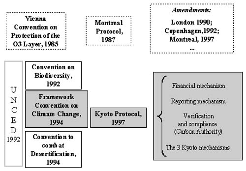
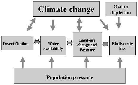
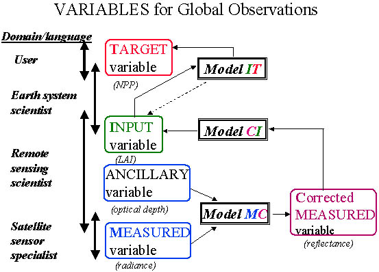
![Figure 1: Steady-state NPP for Australia derived from 185 measurement sites and surfaces of mean annual precipitation, mean annual temperature and soil nutrient status. [Reference: Barrett, D.J. (2000), Steady state net primary productivity, carbon stocks and mean residence time of carbon in the Australian terrestrial biosphere. Global Biogeochemical Cycles, submitted.]](ac668e03.jpg)
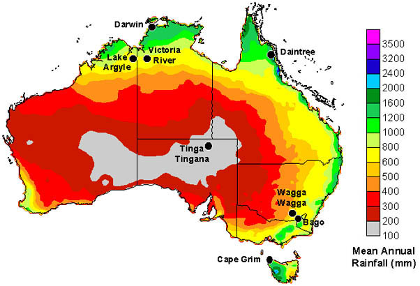
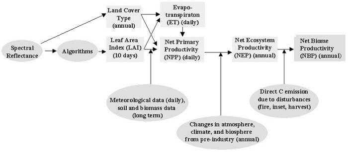
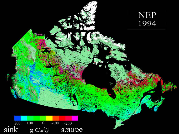
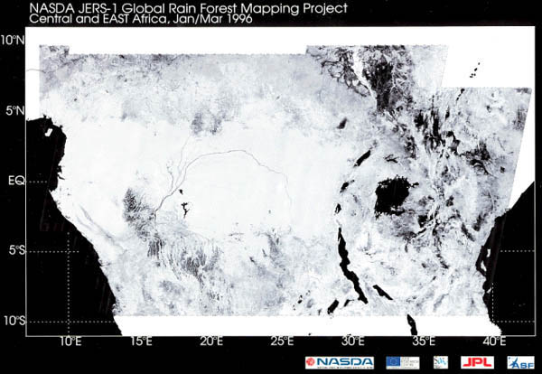
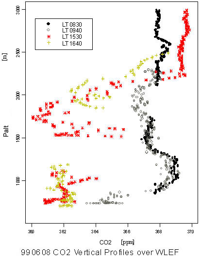
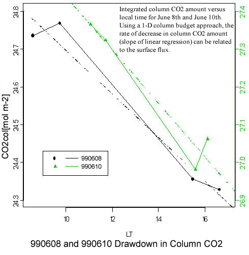
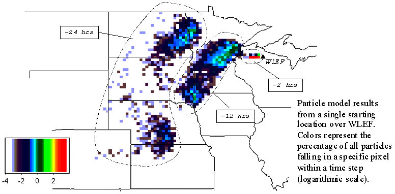
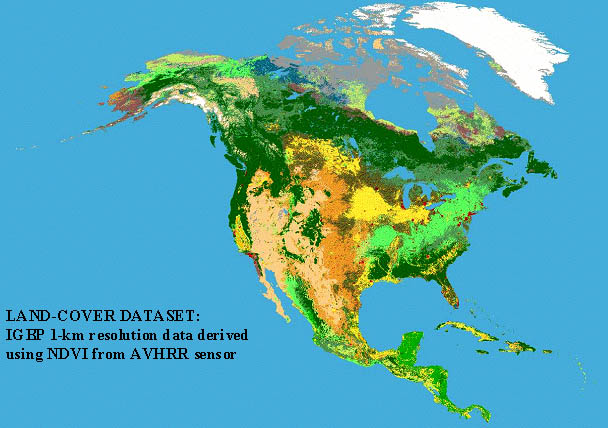
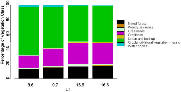
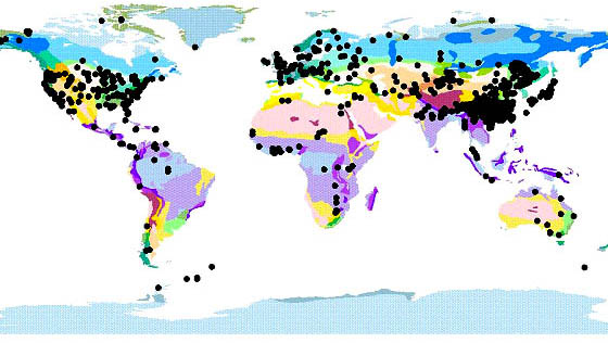
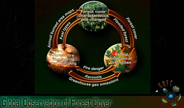