9.1 Ecological Investigation and Modelling
The field of Systems Ecology (e.g., Swartzman, 1979 and Larkin and Gazey, 1982) takes advantage of current powerful mathematical tools and computing technology to model complex ecological systems as mathematical analogues that are intended to preserve the main features of the system being modelled. After a decade or so of this kind of work, a greater understanding of the capabilities and limitations of this approach is now available, and if anything, we are led back to simpler, more robust empirical approaches to food web modelling (see Larkin and Gazey, 1982). A variety of computer models of marine food webs, or at least of trophically interlinked food web components, have been developed. Many of these are complex and are rarely usable in an ‘off the shelf’ fashion without considerable effort in estimating population parameters, but most of them attempt to build up a picture of the consequences of the flow of material or information at a system level, by assembling relatively simple ‘building blocks’ of the kinds discussed in this document. It is our contention, however, that a descriptive phase involving familiarization with the area/habitat in question and the species interactions, is an essential precondition to a sensible modelling exercise, which should then continue to develop in parallel with field observation and experiment.
9.2 Some Indices of Interaction Between Predators and Prey
It could be useful, particularly when comparing the impact of more than one predator on a common prey species, to have some idea of their relative consumption rates. If we assume for the moment that problems of availability of prey to predator are not a problem, then, an annual weighted Index of Predation by predator A on prey C could be defined as:

Obviously, the use of spatial overlap alone is inadequate, if considerations of availability such as vertical distribution (e.g., day-night migrations and predator preference/capture efficiency), considerations are not taken into account. On the other hand, a very limited degree of spatial overlap may reasonably suggest a limited degree of interaction. We may note also that although migratory predators may spend less time feeding on a prey species than ‘residents’, their generally higher feeding rate is important, and this is allowed for in the third term of the above expression.
An index of competition (Ic) between two predators A + B could also be postulated, of the general form:

Comparisons between components of the food web in this fashion should detect pairs of species most likely to be affected by changes in biomass of the other. This could be helpful in preliminary risk evaluation of the possible effects of intensive harvesting of one or more species on those associated with it trophically.
9.3 Estimating Relative Trophic Levels from Food and Physico-Chemical Studies
Food consumption patterns of marine finfish species often show major changes, both in the course of development and on a seasonal basis, in response to abundance, or more properly, to the availability and the size of various food items (Ivlev, 1961). All of these factors make construction of a food web for any given fish community a rather tenuous process, even if all food items can be identified. Of course not all components of stomach contents can be identified, due to problems particularly with fragmentary and digested organisms, and taxonomic problems and losses from the stomach on capture. Clearly, there are also problems, as we have outlined earlier in establishing the trophic level of a given organism in the system. Although the idea of the trophic level is no longer strictly necessary for the food web concept, the relative ‘distance’ above the base of the food web is likely to be given in a very tentative fashion judging from the size and known feeding habits of the species as determined from stomach contents. Thus, after even preliminary examination, a fish may be characterized as a herbivore (grazer), plankton feeder, benthos feeder, or small or large piscivore. This provides.at least some qualitive idea of its relative position in the food web, even if such a preliminary examination does not take into account the “switching” from one prey to another in response to abundance of alternative prey, which Murdoch (1969) argued to be a mechanism for stabilizing prey population sizes.
Isaacs (1972, 1973, 1976) argued that marine food webs (disregarding birds and mammals) are largely unstructured, and are therefore not amenable to trace element concentration study. Results from studies of different coastal ecosystems and the Salton Sea (an inland salt-water lake in the Western United States that has only been in existence for 70 years, which has a very simple food web - see review in Mearns et al. , 1981), tend to support this contention. However, recent very thorough quantitative studies of food habits and incorporated Cesium-Potassium (Cs/k) ratios (Mearns et al., 1981.) and Carbon isotope (13C/12C) ratios (Rau et al. , in press) have shown that very useful information on the mean trophic level of a component can be derived from such data.
Table 6 from Mearns et al. (1981) summarizes the results of computations of trophic levels for three species from the Southern California Bight. The % IRI value refers to the Index of Relative Importance as computed using the methods of Pinkas, Oliphant and Iverson (1971) for weighting the importance of prey species:
%IRI = %F(%N + %V)
where %F = percent frequency of occurence of prey items, %N = percent by numerical abundance of prey item; and %V = percent by volume of prey item. This is a useful weighting factor for determining each prey items relative importance in the diet of a specific predator.
| (1) Assumed or computed prey trophic level | (2) % IRI | (3) (1)×(2)/100 | (4) Computed trophic level = (3)+1 | (5) Traditional trophic level assignment | ||
|---|---|---|---|---|---|---|
| A | Northern anchovy | |||||
| Copepod | 2.0 | 65 | 1.30 | |||
| Detritus | 1.5 | 34 | 0.51 | |||
| Phytoplankton | 1.0 | 1 | 0.01 | |||
| 1.82 | 2.82 | II → III | ||||
| B | Jack mackerel | |||||
| Copepods | 2.0 | 52 | 1.04 | |||
| Unidentified crustacean | 2.0 | 24 | 0.48 | |||
| Unidentified matter | 1.5 | 8 | 0.12 | |||
| Unidentified fish | 3.0 | 8 | 0.24 | |||
| Polychaetes | 2.5 | 5 | 0.13 | |||
| Squid | 3.06 | 1 | 0.03 | |||
| 2.04 | 3.04 | III | ||||
| C | Mako shark | |||||
| Pacific mackerel | 3.54 | 65 | 2.30 | |||
| Jack mackerel | 3.04a | 19 | 0.58 | |||
| Unidentified fish | 3.0 | 17 | 0.51 | |||
| 3.39 | 4.40 | IV → V |
Table 7 from Mearns et al.(1981) shows results from the combined feeding and Cs/K ratio studies for 22 species of pelagic animals from either the Southern California Bight (SCB) or the Eastern Tropical Pacific (ETP). The log transformation of the Cs/K ratios correlates significantly with the computed or assumed values of trophic levels in Table 7, leading the authors to report an average factor of increase of about 2.3 to 2.4 times in the Cs/K ratio at each trophic step. There is a continuum of trophic levels from the assumed levels for zooplankton (of 2) up through the computed value of 5.02 for Carcharadon carcharius, the white shark.
| Species No. | Common name | Locationb | Cs/K × 10-6 | Assigned trophic level | Conventional trophic level |
|---|---|---|---|---|---|
| HERBIVORES (II) | |||||
| 1 | Coastal zooplankton | SCB | <2.07 | 2.00a | II |
| 2 | Oceanic zooplankton | ETP | 3.30 | 2.00a | II |
| PRIMARY CARNIVORES (III) | |||||
| 3 | Northern anchovy | SCB | <1.86 | 2.82 | II → III |
| 4 | Blue whale | SCB | 11.00 | 3.00 | III |
| 5 | Flying fish | ETP | 7.00 | 3.00 | III |
| 6 | Pacific sardine | SCB | 4.02 | 3.01 | III |
| 7 | Market squid | SCB | 2.39 | 3.05 | III |
| 8 | Jack mackerel | SCB | 5.73 | 3.04 | III |
| INTERMEDIATE (PRIMARY-SECONDARY) CARNIVORES (III-IV) | |||||
| 9 | Squid | ETP | 1.94 | 3.52 | III-IV |
| 10 | Pacific mackerel | SCB | 7.23 | 3.54 | III-IV |
| 11 | Frigate tuna | ETP | 8.90 | 3.56 | III-IV |
| SECONDARY CARNIVORES (IV) | |||||
| 12 | California barracuda | SCB | 4.20 | 3.74 | III → IV |
| 13 | Pacific bonito | SCB | 8.01 | 3.80 | III → IV |
| 14 | Thresher shark | SCB | 24.0 | 3.82 | III → |
| 15 | Swordfish | SCB | 12.3 | 3.97 | IV |
| 16 | Blue shark | SCB | 13.2 | 4.00 | IV |
| 17 | California sea lion | SCB | 10.7 | 4.02 | IV |
| INTERMEDIATE (SECONDARY-TERTIARY) CARNIVORES (IV-V) | |||||
| 18 | Yellowfin tuna | ETP | 12.7 | 4.23 | IV ← V |
| 19 | Skipjack tuna | ETP | 8.59 | 4.30 | IV-V |
| 20 | Mako shark | SCB | 19.7 | 4.39 | IV-V |
| 21 | Silky shark | ETP | 22.8 | 4.55 | IV-V |
| TERTIARY CARNIVORE (V) | |||||
| 22 | White shark | SCB | 31.7 | 5.02 | V |
b SCB = Southern California Bight and adjacent waters; ETP = Eastern Tropical Pacific (oceanic)
c Assumed trophic level; all others computed from stomach contentsdata according to methoddescribed in text
Mearns et al., (1981) also report that these ratios do not increase at the same rate for inshore and offshore, or benthic food webs. They also recommend that the dispersion of trophic levels of prey items be recorded, which would indicate the observed trophic spectra each species feeds upon. Such studies, which seem to offer promise for the future, support the concept that variations in time and space are to be expected in the way food webs are structured. Evidently if the methodology described by these workers proves easy to apply, it may provide a further lease of life for the trophic level concept, and for the first time, an objective way of determining it directly. It seems unlikely in the short term, however, to provide a cheap and effective field procedure.
Employing similar logic in studying the 13C/12C ratios in relation to the samples obtained in the Mearns et al. (1981) studies, Rau et al. (in press) report that the 13C/12C ratios also increase with trophic level between the Coastal California and equatorial Pacific waters, and recent work by Mills, Pittman and Tan, 1982 tend to confirm that the “distance” of a given species above the level of primary (plant) production may well be measurable in this fashion. In a parallel sense, it is important to note that some organic pollutants and naturally occurring heavy metals (e.g., mercury in swordfish) also accumulate progressively with higher trophic level and increasing mean age of fish.
9.4 Production, Fishing and Natural Deaths
The production by each species in a food web over a period of time can be defined in a number of ways, which have been summarized by Alien (1971). In simplest terms, if Pn is the net production of species n; Fn the fishing mortality rate it is subject to; and M its natural mortality rate, then, using a simple numerical approach, following Dickie (1972), we can:
Write Pn =  nZn where Zn is the overall species-specific mortality rate, comprising
Fn + Mn , and Bn is the mean biomass of the organism in question. The fraction of Pn
harvested by man (the yield) is defined by:
Yn = (Fn/Zn)Pn = n Fn
n Fn
The fraction consumed by other members of the ecosystems is similarly defined by:
Dn = (Mn/Zn)Pn = n Mn
n Mn
Alternatively, we could define production from the trophic efficiency of a predator population and write:
Pn = KnIn
Where Kn is the overall food conversion efficiency of the predator, and In is the rate of food intake of the predator population. Of course each prey item has a specific conversion coefficient which will need to be estimated with this approach, entailing a considerable amount of experimental work. Nonetheless, a great deal of this work has already been done, so that the variable an (the food consumption rate per unit biomass of predator n), has been documented for a wide variety of species (see e.g., Conover, 1978), and we note here, what will be amplified later, namely that In is defined by:
In = anBn
We could also define production of a predator n+1 in terms of the production of its prey(s) in the trophic level (n) below. Thus, for obligate predator-prey populations in which all prey mortality is due to predation, if food conversion efficiencies of predator + prey can be considered roughly the same:
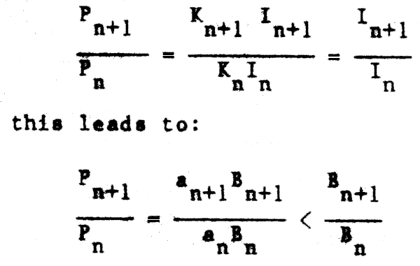
Since, as we note elsewhere, an < an+1, food consumption per unit body weight will tend to decline with increased size of organism. The ratio of production at two adjacent trophic levels should be less than the ratio of biomasses, because not all of the biomass of prey will be consumed by the predator at the next trophic level. However, for other than “stratified pelagic systems”, the proportion of prey species biomass that is consumed by predators is probably rather high for adult fish in marine food webs, even though the particular predator may not always be of commercial importance or even appear eventually in commercial catches. There are obvious dangers with this approach of comparing directly the biomasses of two vertically linked components of an ecosystem to determine predation rate, if not all of the trophic linkages are known, and some more recent concepts have called into question some of the earlier predictions of “simple” trophic concepts as outlined, for example, by Lindemann (1942).
Classically, Lindemann (1942) envisaged animals as belonging to definite trophic levels, thus giving rise to a pyramid (Figure 2): the biomass falling off with increasing trophic level. Much recent research has shown that this need not be the case, given (Isaacs, 1972, 1973) that we have three types of transfer of energy or matter:
k1: conversion of food to living tissue
k2: “loss” of food energy by respiration
k3: conversion of food into a non-living but useable form - e.g., detritus
where k1 + k2 + k3 =1
Under these circumstances, it is possible for predator biomass to be similar to or, even greater than, the biomass of herbivores. For example, if k1 > k2 for predators, and/or k3 > k1 + k2 for herbivores; i.e., if conversion of food into living tissue by predator is efficient (say around 30%), respiration rate relatively low and/or the production of detritus, especially by herbivores, is high so that a high biomass of detritivores exists (which are also fed on by predators), (Platt, Mann and Ulanowicz, 1981), It is possible that the biomass of predators can be high relative to the biomass of herbivores, which is unlike the situation predicted by the simple model. There seems evidence for this situation In some pelagic and benthic ecosystems.
Incidentally, the Isaacs model assuming an unstructured food web, yields reasonable predictions in some other circumstances, and lends some support to the use of compartment models, at least for representing the energetics of ecosystems.
Extension of simple production modelling to multispecies systems: some pitfalls and problems
As noted by May et al. (1979), “A prey-predator system cannot be managed by applying MSY notions to each species Individually”. More generally, from the previous sections, it should be clear that the yield to be expected from a given single species fishery, whether under “equilibrium” conditions or otherwise, cannot be entirely dissociated from the impact on the same stock of the abundance of its predators or prey. The big difference is that usually the natural mortality rate of, and predation on, smaller often immature Individuals is usually highest, while the selective properties of most fishing gear is aimed at the larger, often mature, “commercial” sizes (Figure 38).
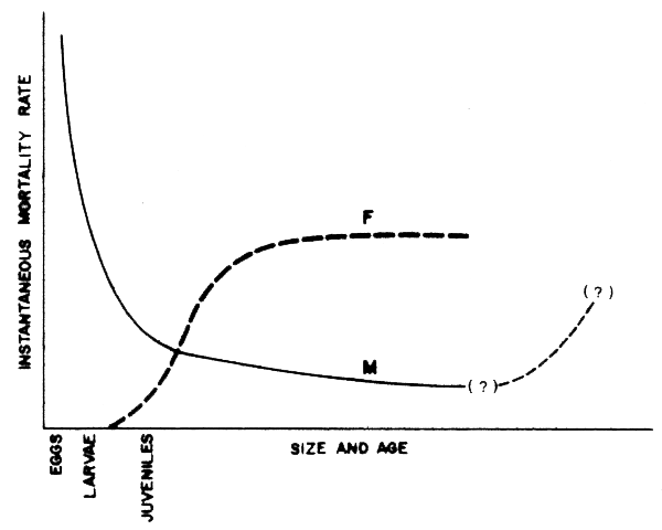
Figure 38 Showing how fishing mortality and natural mortality rates for most commercial fish species caught in area-swept gear (e.g., trawls) have quite different trajectories with size and age. (NB: Survival races for old individuals may decrease, thus showing departures from this generally assymptotic situation)
The consequences of this are not totally evident, except that the recruitment overfishing impact on large, mature members of a stock will likely be more serious than predation on the possibilities of stock replenishment, for the same number of individuals removed. In the simple case however, we can maintain the additive nature of exponential mortality rates postulated in fisheries population dynamics theory (e.g., Ricker, 1975), where total mortality rate Z = M + F.
Some preliminary approaches to modelling catch and effort data from several species in a fishery in combination using the logistic model, have been made, e.g., by Pope (1980), but without taking into account trophic interaction. Such interactions must be important however, and one simple way of visualizing them is provided by extending production modelling theory to include a simplistic formulation of the total production from a species, and its partitioning into fishing yield and natural deaths due to predation. Two interesting features of production curves for a stock under these assumptions are shown by Figure 39 from Caddy and Csirke (1983), namely that as effort and mortality increases towards conditions when MSY (Maximum Sustainable Yield) is being extracted, the total biological production is likely to have also increased, and then fallen with further increases in effort as MSY conditions were approached, unless of course, the total production curve and the yield curve are quite different in shape. If M is high for a stock, this decline in production is likely to begin early in the fishery, to the point that for short-lived species with a high M, yield may not be sustainable, or only at fairly low ratios (F/Z) of exploitation, if predator populations remain high. (Biologically, we may consider such stocks as already significantly stressed by predation to the point of losing some of their “resilience”.) Also the logistic and other production models are of rather uncertain relevance once MSY conditions have been significantly exceeded, and yield becomes more heavily dependent on recruitment and on the ability of a species to maintain to competitive position In the ecosystem at low stock sizes. We should also note (see later) that exploitation of the predators on this stock will influence potential yield of its prey (Figures 40 and 41), although rarely to the extent predicted by simple food webs which assume static linkages.
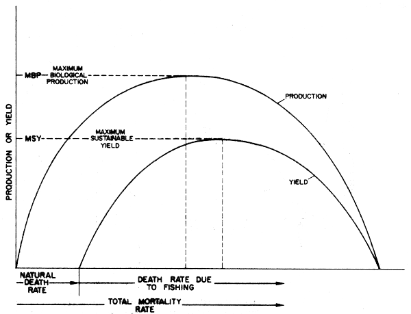
Figure 39 A simple hypothesis as to the response to fishing of total production and yield under the logistic assumption (From Caddy and Csirke, 1983)
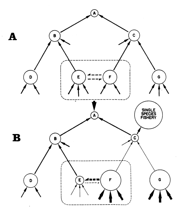
Figure 40 Predator-prey interactions and exploitation (from Caddy, 1984)
Simple unexploited food web for species A-G; solid arrows show flow of biomass from predator to prey with diameter of circles corresponding to species biomasses. (Solid arrows without origin correspond to unspecified prey species, and dashed arrows inside dotted outlines indicate competition between species E and F for space, food, etc.)
A monospecific fishery for species C is now in operation. The thickness of arrows is proportional to rate of flow of material from prey to predator, or (if the arrows are reversed), the degree of control exerted by predator on prey.
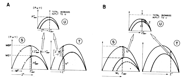
Figure 41 Showing how simple models of total production and fishery yield may be linked to illustrate (in this case), the impact of an increase in effort on one species (T) of a trophically-linked group of commercially exploited species
Another point of this simple model that seems to correspond to reality is that the production from the whole system (yield plus predation) is likely to reach a maximum to the left of MSY - in effect somewhere close to the point of Maximum Economic Yield (MEY) as defined by fisheries economists (from different criteria), or near to the point of F0.1 (now used in many stock, assessments to give a fishing intensity less than fMSY or FMAX Gulland and Boerema, 1973). Preoccupation with fishing prey (forage fish) populations at or around MSY has been expressed, e.g., by May et al. (1979), who note that “preservation of the ecosystem would seem to require that stocks not be depleted to such a level that the populations productivity or that of other populations dependent on it, be significantly reduced”. A somewhat similar concept is implied at the single species level by FMBP (Caddy and Csirke, 1983), which is the fishing mortality rate under logistic assumptions that Maximizes Biological Production (MBP) from a given species. These ecologically-based approaches to resource management are now embraced by at least one international convention for management of marine resources, (that of the Commission for the Conservation of Antarctic Marine Living Resources (CCAMLR) (Table 8).
| ARTICLE I | |
| 1. | This Convention applies to the Antarctic marine living resources of the area south of 60° South latitude and to the Antarctic marine living resource of the area between that latitude and the Antarctic Convergence which form part of the Antarctic marine ecosystem. |
| 2. | Antarctic marine living resources means the populations of finfish, molluscs, crustaceans and all other species of living organisms, including birds, found south of the Antarctic Convergence. |
| The Antarctic marine ecosystem means the complex of relationships of Antarctic marine living resources with each other and with their physical environment. | |
| ARTICLE II | |
| The objective of this Convention is the conservation of Antarctic marine living resources. | |
| For the purposes of this Convention, the term “conservation” includes rational use. | |
| Any harvesting and associated activities in the area to which this Convention applies shall be conducted in accordance with the provisions of this Convention and with the following principles of conservation: | |
| (a) | prevention of decrease in the size of any harvested population to levels below those which ensure its stable recruitment. For this purpose its size should not be allowed to fall below a level close to that which ensures the greatest net annual increment; |
| (b) | maintenance of the ecological relationships between harvested, dependent and related populations of Antarctic marine living resources and the restoration of depleted populations to the levels defined in sub-paragraph (a) above; and |
| (c) | prevention of changes or minimization of the risk of changes in the marine ecosystem which are not potentially reversible over two or three decades, taking into account the state of available knowledge of the direct and indirect impact of harvesting, the effect of the introduction of alien species, the effects of associated activities on the marine ecosystem and the effects of environmental changes, with the aim of making possible the sustained conservation of Antarctic marine living resources. |
The simple approach to biological production modelling implied in Figure 39 in theory could be extended to several species, for example, to a several species Assemblage Production Unit or APU (Figure 41). Here, components of a simple two- prey one- predator system are each considered to be modelled by the logistic model as above. This example illustrates, however, that some features of such a “trophically linked” system may have properties not shown by the individual species. For example, consider Fig. 41, where prey species S is being fished at the point of Maximum Biological Production (MBP), prey T at a lower intensity than this, and predator U at FMSY:
Only a proportion of the biological production of the two prey species S and T, namely
Pu =  (ZiBi -Yi), is supporting the production of predator U.
The apparent paradox occurs when you consider what happens when the fishing intensity on species T is increased, thus reducing the production from species T which is available to predator U, while all other parameters ostensibly remain the same. It soon becomes evident (Figure 41B) that it is not possible to maintain all parameters constant under these circumstances. Changing the point on the production curve for species T must also necessarily change the production curve itself for at least one of the other components, and probably both.
The managers of the fishery on U (and species U itself) appear then to have three options:
Production and yield for species U (and S) may only be maintained constant if U makes up for lost production from species T by switching its feeding to one or more new food items not shown in Figure 41. This is a frequent strategy for many species, especially seasonally, but may not always be entirely successful in maintaining the same level of predator production.
If we specify that total predator mortality (uZMSY) remains the same, and the food requirements are also to remain constant, consumption of alternate prey species S by predator U may have to increase if production of prey T is reduced by fishing. Presumably this will also increase the natural mortality rate of S from Ms in Figure 41A to Ms in Figure 41B. This drops the potential yield of S, since the overall yield to fishing (and, in effect, the exploitation rate on S), is reduced.
Presumably, if strategies 1 and 2 above are not possible, the fishery on U will either produce a lower yield for the same effort (point numbered 1 in Figure 41B),
or:
Effort will increase in response to reduced abundance of U until point number 2 in Figure 41B is reached, where population size and hence food demand of U are reduced.
No final resolution between these possibilities can be generalized upon in such an oversimplified scenario, except to note that a series of continual adjustments of this type must be going on in practise; contributing to the “noise” or even structural instability of many fisheries, especially for species lower in the food chain, and the common departures from “equilibrium production levels” that are frequently noted.
In discussing the quantitative approach to food web analysis, Ulanowicz (1980) notes that four types of flows need to be measured (our qualifications in brackets):
exchanges between (recognized) compartments within the system;
inputs from sources (defined as) outside the system;
usable exports to outside the system (as defined);
dissipation of materials into a form of no use to any system.
The consequence of these points for productivity analysis is that it is probably not valid in most cases to estimate productivity of the food chain in the fashion seen in earlier texts, where “bottom-up” calculations were based on an overall estimate of primary production, to which were applied successively loss rates for herbivores, primary carnivores, secondary carnivores etc., of roughly 90% to eventually evaluate potential fish yield. Clearly, this type of calculation is incorrect in several ways:
the estimates of biomass lower down in the food chain (especially for primary predators) are likely to have wide margins of error;
the efficiency of transfer of biomass is not a constant;
marine species normally move upwards in trophic chains in ontogeny;
leakage occurs to undefined species;
the effects of detrital recycling is not taken into account (see e.g., Newell, 1984).
There doesn't seem to be any escape from the conclusion that the main components of the system need to be identified individually, and the actual food linkages, and where possible, the order of magnitude of biomasses and transfers, need to be estimated in order to use a subset of the food web as a basis for intelligent hypothesis and experimentation.
Simple trophic analysis of a food web
As a first approximation, it may be convenient to proceed directly from a preliminary prey-predator contingency table (e.g., Fig. 39A) to construction of a tentative food web (Figure 39B), even though estimation of the rate of feeding of predators in absolute terms requires considerable knowledge of ingestion, digestion or egestion rates, both as a function of environmental factors, and of type and abundance of food. These latter factors will be touched on later, but for the moment the assumption is made that the relative volume of identifiable food contents per predator body weight, is an index of their fraction in the total diet. This assumes that the sample of stomachs is properly weighted both for diurnal and seasonal factors, and for the distribution and relative abundance of the different size groups under investigation.
To some extent a preliminary trophic classification of this kind is possible by reference to the literature, although information is surprisingly sparse on the diets of many marine fish species.
“Stomach content analysis” (including intestinal contents) is the principal method available to the field worker with limited facilities for intensive laboratory or field studies. This methodology and the data it generates has been inadequately utilized to date, largely we believe because of uncertainties in the interpretation of the large volume of data that can be rapidly obtained by this method. To a large extent this is also because methods of population analysis until recently have placed inadequate emphasis on multispecies approaches and species interactions.
One suggested approach to analyzing the preliminary food web is given below in five steps, illustrated by means of a simple hypothetical example. It is assumed here, as a simplifying assumption, that the food requirements of a species are homogenous. In reality, it would be necessary for most species as we have seen, to divide each up into two or more size or age categories corresponding to the different trophic levels occupied in the life history; (or treat each of these as separate groups of organisms):
Step 1: Preparation of primary contingency tables of stomach contents for the main predators showing mean weight (volume) of prey in the stomach as a fraction of predator body weight (Figure 42).
| PREDATOR | |||||
| 1 | 2 | 3 | 4 | ||
| 1 | 0.024 | 0.030 | 0.030 | 0.040 | |
| PREY | 2 | 0.050 | 0.020 | ||
| 3 | 0.019 | ||||
| 4 | 0.001 | 0.080 | |||
| UNIDENTIFIED FOOD | 0.003 | 0.030 | 0.040 | 0.031 | |
Figure 42 Matrix of food consumption data for four trophically linked species showing stomach contents as percentages of body weight of the four components
Step 2: A preliminary food web is constructed (Figure 43).
Step 3: The proportion of identifiable stomach contents per item is calculated.
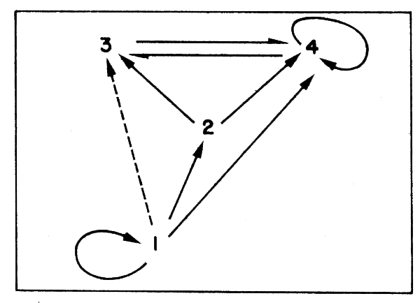
Figure 43 Simplified food web based on Figure 42
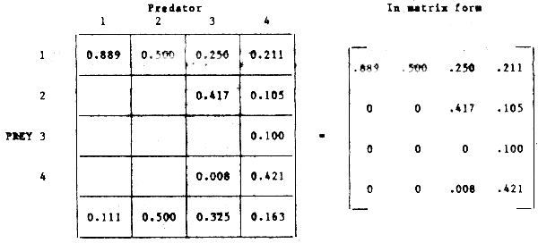
(Unidentified stomach contents either are not included in the matrix , or allocated proportionally to recognizable items).
Step 4: Correction for feeding, egestion or digestion rate, (if possible by post-multiplication of the above matrix by a diagonal matrix B containing the estimated feeding rates):
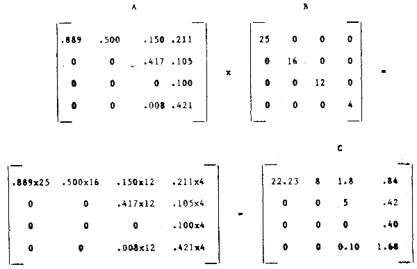
The last matrix is then our best estimate of the food consumption per unit time per unit of predator body weight.
Step 5: Absolute food consumption can then be obtained per unit time by post multiplication of the above matrix by a diagonal matrix containing the biomass of each predator:
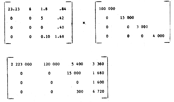
This can be condensed further to estimate absolute food consumption by each predator per unit time T as a horizontal vector:
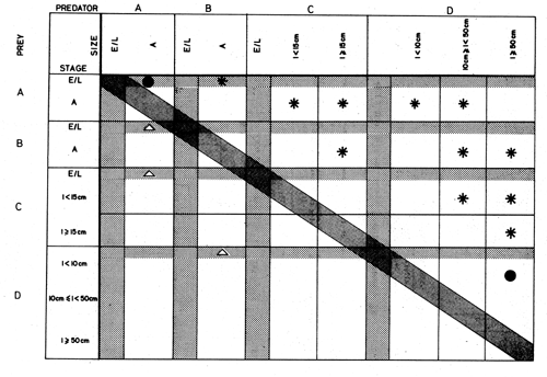
Figure 44 Prey-predator contingency table for part of a hypothetical neritic food web, including two small pelagic species (A, B) for which eggs and larvae (E/L) are recorded separately from adults (A), and two higher trophic-level predators (C, D) for which eggs and larvae and two or three trophically relevant size categories are recorded separately. Predation is shown by an asterisk; cannibalism by a solid circle. Note that reciprocal consumption of the larvae of adult predators by small pelagic “prey” falls below the matrix diagonal (triangles)
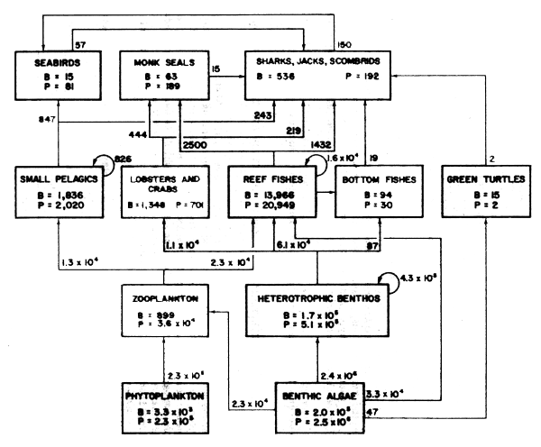
P= annual production; B= mean annual biomass (kg/km2); values with arrows are amounts consumed of lower trophic level production
Figure 45 Flow of materials through a marine ecosystem (1 200 km2 in area) in the north-west Hawaiian Islands (Redrawn from Polovina and Ow, 1985)
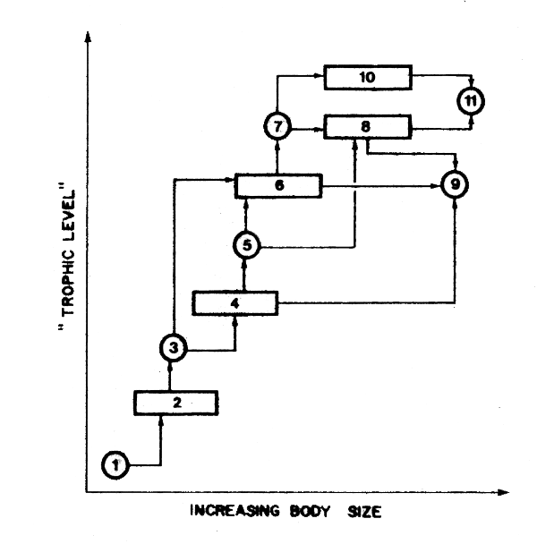
Figure 46 A food chain showing the strategy of calculation suggested by Borgmann (1983), which postulates “hypothetical species” (circles) that are effectively of constant size and are used to simplify the mathematics of computation of production when real species (rectangles) actually vary in size
Predator
| 1 | 2 | 3 | 4 |
| 2 223 000 | 120 000 | 20 700 | 13 360 |
or total amount of each prey consumed by a vertical vector:

One aspect of marine food webs that is not readily represented by the above simple matrix approach needs mention here, and is illustrated in Figure 44, namely the fact that there are often significant changes in trophic preference in the course of the life history. A modified contingency table such as that shown may then be useful for representation of different life history stages in the context of trophic interactions.
Simple Ecosystem Models
The ECOPATH model is one of a number of simple compartment or box models which attempt to simplify the complexities of massive food webs by placing food web components into major categories with known linkages (see Figure 45 from Polovina and Ow, 1985), for each of which estimates of total production, predator biomass and catch are available. The model requires that equilibrium conditions exist, when estimates of production (such as those measures suggested by Allen, 1971), and constant species-specific values of M and F derived from population assessments also apply. The importance of the assumption of equilibrium is that the biomass budget equation (for all prey species i = 1, 2, 3…n) can then be simply defined as:

and then used to estimate unknowns. Estimates of the rate of flow through the food web are only strictly valid under these circumstances, (as of course, is the assumption of constant natural mortality rates). This poses some serious problems for the general applicability of such modelling approaches, but this type of model still seems to offer a first entry into what is, as we have seen, a complex multispecies ‘landscape’. One other problem faced by this approach is the difficulty of dealing with intraspecific variations in diet with season and size. One approach that offers a partial solution to this problem is suggested by Borgmann (1983) where size ranges of species are extended, namely, to postulate hypothetical species of a fixed size that allow the some general increase in body size with distance upward in the food web to be treated more easily (Figure 46).
It is not apparent, however, that this device allows for those changes in size range that occur upon exploitation.
The useful, if rather over-simplified concept of the r-K continuum of life history strategies, first coined by MacArthur and Wilson (1967), has proved valuable in attempting to integrate life history information in relation to the role of a species in the marine ecosystem, even if it is difficult to quantify in practical terms. Stated simply, it is postulated that two major evolutionary strategies can be recognized, r and K selection, each of which is particularly adapted to characteristic patterns of change in the biotic or abiotic environment. As we shall see, there are problems with the oversimplification, but it is useful for the student to be aware of this distinction.
Two main modes of selection are postulated to occur, as suggested by the Verhulst-Pearl or logistic equation:
dN/dt = rN - (r/K)N2
where r is the maximum rate of increase that a population of initial size (N) exhibits when released from exogenous limitations (i.e., not food limited, little predation, etc.), and K is the carrying capacity of the system, equivalent to the virgin biomass or carrying capacity of the environment in the usual fisheries formulation. Pianka (1972) notes that although some species are particularly adapted to rapidly occupying vacant spaces in the ecosystem (r strategists), others are better adapted to slowly increasing their share of the resources of the system under conditions of high competition (K strategists).
The r- strategists are species adapted to living in environments where there is a high density-independent mortality rate. Such areas include for example, upwelling zones, and those high latitude seas where (for annual species at least), seasonal periods of high food abundance are followed by periods of relative scarcity. These species tend to allocate a greater proportion of their resources to reproduction, having in consequence a high gonadosomatic ratio and birth rate, a short life span, as well as being in general relatively unspecialized, especially for example in feeding habits. Population size is generally prone to high fluctuations in numbers (e.g., Engraulid and Clupeid species).
By contrast, K strategists are adapted to living in environments where intra-and interspecific competition is high. These tend to be mature, relatively stable environments, such as coral reef and mangrove areas in the tropics. There is consequently a high degree of selection by means of density dependent factors, and these species have evolved to allocate a greater proportion of their resources to non-reproductive activities promoting individual survival. They are consequently relatively specialized in their trophic activities and other behaviours, and in general are longer-lived, less fecund, and less prone to major short-term changes in population size (e.g., sharks and whales: see Table 9 for a review).
| Characteristics | r-selected | K-selected |
|---|---|---|
| Climate | Usually variable and/or unpredictable | Fairly constant and/or predictable (or species shows migratory behaviour) |
| Risk of natural death | Often high or catastrophic: largely independent of population size | Death rate is more scheduled and dependent on population size |
| Population size | Variable in time, non-equilibrium conditions prevail; occupies eco- logical vacuums but rarely reaches the carrying capacity of the environment; recolonizes habitat each year | Fairly constant in time, at or near carrying capacity of environment; no recolonization necessary of saturated communities |
| Competition between species and within species | Generally lax | Usually keen |
| Length of life | Short (usually one or less than one year) | Longer (usually more than one year) |
| Natural selection in favour of: | (1) Rapid development (2) High rate of population increase (3) High rate of egg production (4) Small body size (5) Single reproduction (6) Less emphasis on behavioural and morphological characteristics to increase individual survival survival habits | (1) Slow development (2) Low rate of population increase (3) Low rate of egg production (4) Large body size (5) Multiple reproduction (6) Behaviour and morphology assures good individual survival, e.g., territorial behaviour, spines, special dentition and special feeding habits |
| All above lead to: | Productivity | Efficiency |
In his general review of the field, Pianka (1970) notes that in terrestrial systems there is a very clear distinction between the two strategies, and that in fact, for terrestrial animals this results in a clearly bimodal distribution of sizes, between small (predominantly annual) arthropod-dominated species, and larger, often perennial vertebrates; epitomizing in a rather clear-cut way the distinction between the two types of selection. He notes that to survive with a generation time longer than one year in a strongly fluctuating seasonal environment, a species must be adapted to the full range of ecological conditions encountered during a year. This is in contrast to annual species, which typically encounter only a limited range of seasonal conditions at any given life history stage, to which they can be perfectly adapted, and if necessary can pass the remainder of the year in an inactive “resting” stage, as eggs, spores, larval forms, etc. This suggests that generation times exceeding one year may be the threshold event in the evolution of a species, and will be characterized by a rather drastic shift from r to K selection modes. However, Pianka notes that fish show the full range of the r-K continuum, probably because (especially in tropical environments), seasonal changes in the ocean are strongly buffered, except for regions of environmental instability (e.g., upwellings, intertidal and estuarine regions) where it may be expected that r selected species are dominant. A summary of the main characteristics of r and K species is given in Table 9.
More recent work has cast some doubts both on this duality, and on the logistic assumptions that underlie it: for example, the concept of an equilibrium value for the carrying capacity K of an ecosystem requires some careful consideration: the known variations in carrying capacity K in a given area, with time, causes one to wonder whether in managing such resources, one should adopt the usual steady-state equilibrium approach, the open-system non-equilibrium approach, or perhaps some combination of the two (Caddy, 1984). The answer to this question, though far from clear-cut, depends on the time scale being discussed: even “stable” populations, over a long enough time scale, show departures from average landings as calculated over the medium term.
In the fisheries literature, the steady-state approach is the one most often assumed to apply, however, and because the different levels of harvesting can be quantified, this allows one the opportunity to test the relative effect of different perturbations on the system being examined. It is primarily due to this useful characteristic that approaches based on the equilibrium assumption have dominated the literature. However, a description of the open system, non-equilibrium approach (Johnson, 1981) shows that it can be equally valid to consider ecosystem dynamics as a series of perturbations, rather than as a system in equilibrium, and the application of this alternative hypothesis in fisheries is discussed in Caddy (1984) and followed up by e.g., Allen and McGlade, 19861. The logical differences are fundamental, but this duality in approach is a common denominator of nearly all fields of science which seek statistical predictions of likely future states of a system, e.g., in thermodynamics, small particle physics, the functioning of nervous systems, etc.
There are numerous examples of rapid changes in state occurring in marine biology: the abrupt transition of larval forms seen in many marine organisms at various stages in development is one example. Most fish start life as an independent egg adrift in an uncertain environment with few adaptations other than physiological for survival; therefore, their common “objective”, expressed anthropomorphically, is to become independent of local environmental limitations by becoming mobile. This requires that they proceed as rapidly as possible through the developmental stages leading to increased mobility. This is classic r selection. Some other fish bear live young, which are already quite mobile at birth: a classic K selected process. However, fish that grow to large sizes from small eggs often become characteristically K strategists to the point of expending far more of their energy in activity than in reproduction. The oceanic nomad species are good examples (e.g., tunas, dolphin fish, billfishes).
Clearly there is no set of either-or conditions in regard to r and K labelling of fishes. This makes it quite difficult to quantify the utility of these concepts in application to practical ecological problems. However, there are interesting relationships between the intrinsic rates of increase, r, and population density. For example, looking a little further into the implications of the mathematical theory mentioned earlier, if we plot the rate of increase in population against population density as in Figure 40, we see that to the left of some density, X, the r-strategist is at a competitive advantage, while to the right, the K-strategist is favoured. It is interesting to note here that the plot of rate of increase against density in Figure 47A is functionally equivalent to a stock-recruit model, and further, although this analogy should not be carried too far, than there is a resemblance between the curve for r-strategists and the so-called Ricker Spawner-Recruit (S-R) curve, Figure 47B while that for K-strategists resembles the so-called Beverton and Holt S-R curve (Ricker, 1975). An example of the former in the marine sphere is the anchoveta, typically a short-lived opportunistic species, and of the latter, the North Sea herring. This latter is a relatively long-lived species, formerly occurring in great abundance, but with a demonstrated vulnerability to density-independent mortality effects. These latter we may consider to include human predation by fishing, especially on spawning grounds. In herring, fishing effort remained high despite declining abundance, in part because the species is vulnerable since it occurs at a uniformly high density on the spawning grounds, whatever the stock size. The relationship between the form of the hypothetical spawner-recruit curve and the concept of r and K selection is logical, since both deal with the rate at which a stock replenishes itself under different densities. Obviously, with no parental stock, there will be no reproduction, but for most species it is still far from obvious what is the relationship between parental stock size and the numbers of progeny produced. In the S-R relationships populated to date, the number of recruits drops off with biomass or density since as is inevitable in a finite habitat, there is only limited space and food for a certain number of individuals. Line A-B in Figure 47B would only then be approximated in a continually expanding environment. Expressed somewhat differently, although we should ideally try to describe what is the relative contribution to reproductive success of parent stock size, environment, and interaction of recruits with other organisms (predators or competitors) in the ecosystem, this will be no mean task, and presupposes first that we have a good understanding of the life histories of the key component, and their interrelationships.
Reviewing the field of density-dependent recruitment is unnecessary here, but a few of the underlying concepts from this extensive literature (see Ricker, 1975 for an introduction), need to be placed in an ecological context.
The overall carrying capacity K of an ecosystem can only be defined in the context of its basic productivity, and the relative efficiencies of population growth and food conversion, and hence abundances, of the component species within it. The thermodynamics of energy acquisition and conservation is the fundamental ‘preoccupation’ of species in their life history strategies, but this is expressed through the activities of work-growth-reproduction and relocation, so that the fundamental problem for an ecologist is of defining, measuring and monitoring these processes. To assume for a species or stock a simple relationship, where recruitment is only a function of parent stock size, is to start well above the relevant levels of interaction, and is unlikely to yield satisfactory insights into the dynamics of either ecosystems, or even of one component population.
The concept of the ecological niche in the marine environment
In many, if not most oviparous species, the habitat for larval survival is so specific that the carrying capacity of that subset of the species' overall habitat or ‘niche’ may well be the main constraint on the species in question. Salmonids (Ricker, 1975) and engraulids (Lasker, 1978, Bakun and Parrish, 1980, Sharp, 1980b, IOC Workshop Report No. 28), appear to exemplify these constraints in action.
The following enlightening discussion of the likely impact of multiple and overlapping eco-logical niches for various marine fish species, on our perception of “competition” for food, is taken from Jones and Henderson (1980):
“The possibility of larval niches of different sizes, as well as adult niches of different sizes raises other considerations in connection with the full utilization of food resources. Thus if the population size of a particular species is regulated prior to the adult stage it may appear possible to have a non-limiting food resource for the adults. This however, must be a short term viewpoint. In the long term, other species may be expected to take advantage of any surplus food, and eventually all resources should be fully utilized. The problem then is to explain how it is possible for the adult population of any one species, to expand suddenly, due to the influence of one or more good year-classes.”
An understanding of how this might be possible comes from a consideration of larval and adult habitats as separate; each with its own competitors and interspecific competition. Thus, larvae or juveniles of a species exploit a particular resource, and the adults exploit a different one, consisting of larger-sized food particles. If the adult resource is not fully utilized, there is room for the adults of a second species (Y) to share the adult resource. However, it should be possible for both species to co-exist providing their larvae exploit different resources. This process of adding species can be expected to continue untill all the adult food resource is completely utilized, and all larval niches are occupied. (We may note that the addition of “new” species in this way is occurring continuously by evolutionary processes).
Continuing, Jones and Henderson (1980) note that “In a multispecies situation of this kind, … total recruitment is less variable than the recruitment of individual species. A temporary expansion of one species could then be offset by a temporary decrease of other species. This is an attractive argument since it provides an explanation of how it is possible for the diets of many fish species to overlap, without competition reaching a level at which one or more species is eliminated. It also explains how it is possible for the adult stock of any one species to increase significantly, due to one or more good yearclasses, without exhibiting evidence of significant resource limitation. Resource limitation of adults will depend on the combined biomass of all species sharing the same resource, and this may vary very much less than the stock sizes of the separate species. The assumption that there is an upper limit to recruitment due to resource limitation during the early life is attractive because it makes it possible to understand how a relatively large numbers of species might co-exist. Given differences in time, as well as in space, the potential number of larval ecological niches must be very much larger than the potential number of adult ecological niches.”
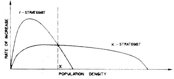
Figure 47A Postulated relationship between population size and rate of population increase for r- and for K-strategists
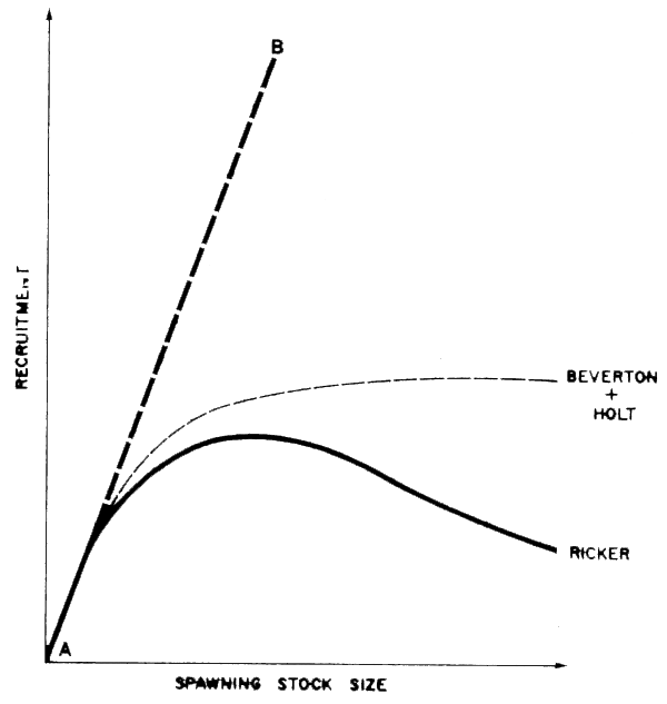
Figure 47B Two relationships between spawning stock size and subsequent recruitment in common use. (Line A-B is the trajectory that would apply if recruitment were proportional to stock size.) See Ricker (1975( for details
Given that the absolute number of fertile eggs produced puts a ceiling on the possible size of a new generation, the question of where and when they should be laid seems the next logical question to ask. Homing species and localized populations are both tuned by selection to “fit” the occupied habitat, or become extinct. The significance of this statement is often forgotten until a massive change is observed in the range, distribution and abundance of a species or groups of species. Recently Parrish and MacCall (1978), Csirke (1980), Grainger (1980), Iles and Sinclair (1982), Sharp (1980a; 1980b), Bakun and Parrish (1980) and Sharp and Csirke (1983) have documented and tried to elucidate the time-space and ecological implications of physical and biological variations in the environment and their effects on population level variations and recruitment success, as well as on distribution and abundance. The problems of time and distance scales need resolving before useful questions can be answered (Sharp, 1980a; Fasham, 1978).
In general, the perspective emerging from even this brief discussion, is that for many marine species with multi-stage life histories, the idea of an ecological niche as the sum of all physical and physiological influences on the species, becomes virtually impossible to define in quantitative terms. It is perhaps also incorrect axiomatically in its implication that each species is unique in its position in the ecosystem: a growing realization of the wide degree of overlapping in life history stages and their trophic preferences is perhaps a better description of current thinking in this area.
A series of questions, and a brief illuminating discussion of the ‘multiple’ nature of niches in the marine ecosystem is extracted from Jones and Henderson (1980):
“For a long time, fishery biologists have been speculating about the dynamics of fish recruitment and the method of population regulation in teleost fishes. Associated with this problem are important management questions, such as “how hard can a particular stock be exploited before there is a risk of recruitment failure and a collapse of the fishery?”
There are also important ecological questions such as:
“How are fish populations regulated, given that there is apparently no correlation between stock size and subsequent recruitment?”
“At what stage in the life history is the level of recruitment determined?”
“How is it possible for a good yearclass, to lead to a significant increase in adult stock size, without the individuals in that stock showing obvious signs of resource limitation?”
“How is it possible for so many species (particularly in tropical waters) to co-exist, when there is apparently such a large overlap in their diets?”
“In the present state of knowledge, it is not possible to arrive at defnite answers to any of these questions. All that can be done, is to provide a framework, within which plausible answers to these questions suggest themselves.”
In relation to the definition of recruitment level and stock size, Jones and Henderson (1980) note that: “Since different life stages exploit different food resources, it becomes important to distinguish between the average level of recruitment, and the average size of the stock. Thus, average recruitment (R) each year, should be largely determined by the size of the juvenile food resource but, average larval production (L) each year is likely to be determined by the size of the larval food resource.
Adult stock size (A) on the other hand is more likely to depend (in the long term) on the size of the adult “ecological niche” than on the number of recruits produced annually.” In relation to the questions of resource rarity and dominance they also note that:
“Where there are many species, it seems likely that those that succeed in exploiting large resources as adults, will also succeed in exploiting large resources as larvae and juveniles.
In this context, a large resource might not only mean a large geographical area, as suggested by Iles and Sinclair (1982) but also an extended spawning period, or both.”
r-K-selection theory and stock recruitment
Garcia (1982) has documented the illogicality of assuming a single stock-recruitment relationship for penaeid shrimps, a group where the adult and earlier stages are ecologically separated, hence few direct intraspecific effects beyond egg production can reasonably be assumed. This example shows in the simplest case of an annual (r-strategist) that the environmental conditions during spawning and recruitment can be at least as important as stock size in determining the size of the next generation. There are clearly also other parameters which may determine the realization of recruitment potential, by affecting processes such as transport, predation, etc., and which modify the potential represented by the viable, fertile eggs produced by the spawning stock.
The limited utility of the single species spawner-recruit paradigm becomes even more apparent when one tries to describe the effects of one species' failure to take advantage of a series of ecological blooms in its prey species, or in the prey of its larval form. This failure may perhaps be due to low predator abundance, hence to a poor ability to take advantage of opportunities. These “missed opportunities” may well (in fact, are likely to), be taken up by another (competitor) species, yielding a bloom in this normally subdominant species which in this context can be regarded as an r-strategist. Perhaps the sequences of anchovy-sardine blooms evident in the literature on pelagic fishes represent just such scenarios (Soutar and Isaacs, 1974). Skud (1982) has focussed his attention on the impact of such changes in species dominance in modifying the correlation between ambient conditions and the population characteristics as sampled by fisheries, of the species that alternate in dominance.
From analysis of fish otoliths in bottom sediment cores, it seems that such species change-overs were occurring regularly in areas where high levels of pelagic production are now the case, for tens of thousands of years prior to human intervention in the form of a fishery on the species components (Devries and Pearcy, 1982). This raises the question, not yet adequately answered, of the relative importance of high fishing intensity and environmental instability in determining population changes, particularly for species such as the Peruvian Anchovy (The Costa Rica Symposium: Sharp and Csirke, 1983).
r-K selection theory and natural mortality rate, M
A further relationship between r and K theory and conventional fisheries dynamics, concerns the natural mortality rate, which may be considered as being inversely related to the individual fitness of an organism to survive.
A study of a limited number of (unfortunately, largely arctic-boreal) fish species (Gunderson, 1980), supports the prediction from r-K selection theory, that natural mortality should increase as one moves across the spectrum from K-strategists to r-strategists.
It was noted that there have already been a number of attempts to estimate this very difficult and important parameter (M) indirectly from its correlations with various other more easily estimated parameters. Thus, mainly for terrestrial organisms, a strong positive (nearly linear) correlation exists between the logarithm of body length and the logarithm of generation time (i.e., in conventional fisheries terminology,
log (L00) = a + b log (1/M)
but Gunderson (1981) found body length to be the weakest variable for predicting M of the four variables he used, the others being:
Age at 50 percent female maturity (Tm);
longevity (the age T.01 by which abundance has declined to one percent of the average numbers recruited under unexploited conditions);
The von Bertalanffy growth rate, K;
Gonad index (GI) defined in its simplest form as gonad weight for mature females. (This index is better than body weight as a measure or fecundity, since it takes into account both spawner population and number of eggs produced per female).
This last measure (GI) proved to be the single best correlate with M of those considered, so that the following regression was highly significant:
M = 4.64 GI - 0.370
The addition of the second most useful variable (T.01) in a multiple regression to predict M, only decreased the standard error of the estimate by a further 12 percent.
As noted by Beverton and Holt (1959) and Southwood (1976), the von Bertalanffy growth constant
K' for individual growth (not identical with the Verhulst-Pearl K!) is a good correlate of M within
taxonomic groups, as would be expected from r-K selection theory, since short-lived animals
generally have high metabolic rates and individual growth rates; once again well correlated with K.
However, correlation between the two variables is rather poor when members of more than one
taxonomic family are included. Nonetheless, Pauly (1980) using a multiple regression approach
similar to Gunderson's, found that a first estimate of M could be gained from a knowledge of K, Loo
and mean environmental temperature ( ), and suggested formulae for obtaining M from a knowledge of
these. His multiple regression equation was given earlier.
Definition of  for some of the larger, especially the mobile species in Pauly's list is quite
arbitrary however, and the wide variance around the relationship must encompass not only a significant
measurement error, but also variability due to fluctuations in predator-prey relative abundance
and prey availability which are not included within the three independent variables. It is
therefore somewhat surprising how well this equation succeeds in establishing an “order of magnitude”
for the population mortality rate.
Gunderson's equation using GI cannot be used as given for tropical species, both because it would extrapolate beyond his very limited sample (very few of the relevant data sets are available for tropical species), and also because (multiple) spawning of tropical species often occurs over a longer period of the year than for temperate species, so that the Gonad Index would have to be adjusted for repetitive spawning to be a good index of either M, or the species position on the r-K spectrum. This criticism also invalidates the equation of Rikhter and Efenov (1976) for use in tropical waters. A comparison of known M's with values of E, would be needed, (where E = number of eggs shed per mature female) x fo: fo is the mean number of spawnings (including partial spawnings) per year by mature individuals. This approach would be of interest, but for the moment the necessary data sets are not available to test it.
r- and K-selection and the “ecological niche”
The concepts of species interaction and competition are also easily placed in the context of r- and K-selection theory: competion for a limited supply (of space, food, etc.) will inevitably increase with crowding, so that one can predict that the maximum tolerable niche overlap will be greater in relatively saturated communities (i.e., K-selection conditions), and one may expect more exotic adaptations, behaviourally and in terms of body structure, to occur as species diversity increases.
As noted earlier, Baisre (1985) described in sequence three Cuban ecosystems (estuarine, reef-associated and oceanic), in terms of the decreasing influence of land [Figure 48(A-C)]. With distance offshore, dissolved nutrient levels diminish, “particles” (organisms) increase in size, as does the index of diversity and the maturity of the communities, although Baisre notes that some organisms may move offshore along these gradients in the course of their life histories. Concomitantly, he speculates that a move from r- to K- life cycle strategies occurs as unit productivity decreases. An even more sweeping generalization, which nonetheless has a degree of truth, is that while spawning and hatching tends to occur for many species in stable environments such as eel grass beds (see Pollard, 1984) where natural mortality is reduced, larval and/or juvenile life histories may take place in more unstable environments where the food supply is greater.
Judged from the preceding account, r-selected species would seem less manageable than K-selected ones. This conclusion must be regarded with caution, however, because such a simple two-way classification does not take into account that we may be talking about a function of environmental instability as opposed to just a function of life history strategies. Caddy (1984) notes that “it seems quite possible for a short-lived r-selected species to achieve and maintain dominance in a stable environment if the population of K-scheduled competitor species is kept low by fishing.” Some cephalopod and shrimp populations seem to illustrate this, even if longer-lived finfish components have been cropped down.
An alternative classification to r-K theory has been proposed by Kawasaki (1980) that leans heavily on Japanese experience in N.W. Pacific Ocean. This is shown in Table 10, where a long-term history of fluctuations in production tied to the Kuroshio Current system provides an interesting perspective to the opportunistic and varied approaches to a wide resource basis adopted by the Japanese fishing industry.
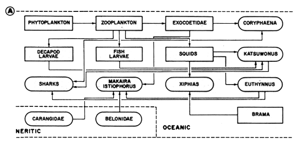
Figure 48A General scheme of feedings relationships in the oceanic water complex. Data from various authors cited by Baisre (1985)
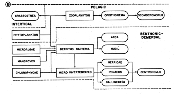
Figure 48B General scheme of feeding relationships in the littoral estuarine complex. The names in circles correspond to species or commercial groups. Information from various authors given by Baisre (1985)
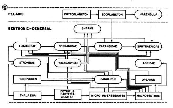
Fig. 48C General scheme of feeding interrelationships in the ecological complex of reefs and turtle grass beds. Data from various authors cited by Baisre (1985)
In Kawasaki's scheme, two main and two subsidiary classifications of species are proposed: Type II being similar to the K-selected category above, except that number of eggs produced per spawning is high and includes, as examples, cods and flatfish (e.g., Type 4). Being generally high in the food chain as adults, these species may be considered manageable by conventional yield models, with equilibrium concepts being largely applicable.
Type I is divided by Kawasaki (1980) into:
Type IA - small short-lived species with low individual fecundity but very early maturity, early spawning and hence high rates of population increase. These species (e.g., saury, squid and sand eel) tend to inhabit irregular variable environments and show high population variations, making them essentially very similar to the r-classification prescribed earlier (except for their low fecundity), and they may be considered non-equilibrium stocks where pulse fishing may be the only way of harvesting the stock without excessive wastage due to natural deaths in good years, but where effort will have to be directed elsewhere in poor years. Here the manager is faced with the conflicting considerations of deciding between a high enough effort level that reduces wastage and a high probability that alternative fleet deployment to other resources will be needed if population crashes occur, as usually seems to occur at some point in time with this type of stock (e.g., Figure 18).
Type IB - Here we have stocks adapted to areas with long-period fluctuations or cycles in suitability of the environment for stock recruitment within the cycles. This group is somewhat intermediate between the other two in that life spans are long enough, but age at maturity is generally early, with multiple spawnings and moderate fecundity allowing a rather high rate of build-up of population biomass over the medium-term (5–10 years?) period of favourable conditions, and with sufficiently long life span for some individuals to survive to the next favourable period (e.g., sardines, herring).
| Type I | Type II | |||
|---|---|---|---|---|
| Sub-Type A | Sub-Type B | |||
| Environment | Variable and unpredictable | Stable and predictable | ||
| Irregular variation | Long period | variation | ||
| Recruitment | Variable | Stable | ||
| Irregular variation | Long period variation | |||
| Resources | Reproduction | Growth and maintenance | ||
| put into: | Reproduction only | Reproduction % maintenance | ||
| Lifespan: | Short | Long | Long | |
| Growth: | ||||
| Growth rate | Moderate | High | Low | |
| Maximum size | Small | Moderate | Large | |
| Reproduction | ||||
| Age at first maturity, | Very low | Low | Quite low | High |
| Fecundity | Low | Moderate | High | |
| Intrinsic rate of population increase | Very high | High | High | Low |
| Early survival | Variable | State | ||
| Trophic level | Low | High | ||
| Typical species | Saury, sandeel | Sardines, herrings | Cods, flatfishes | |
| Appropriate management measures | Catch forecasting and monitoring (+ pulse fishing?) | Recruit forecasting & yield/ recruit assessment & MSY fishing? | Equilibrium yield assessment, steady state (F0.1) fishing. | |
The interesting question which it is obviously most difficult to answer from short term research, is the extent to which an ecological system or community is subject to changes or fluctuations over the long term. Perhaps one of the first systems where repeated “switching” between two dominant ecosystems has been studied in some detail is that referred to as the “Russell cycle” (see Cushing 1982 for a description and references). Briefly, a change in ocean circulation causes major changes in characteristics of water masses, plankton and dominant pelagic fish stocks in the English Channel and Southern North Sea: principally between dominance of pilchard and herring stocks. Similar events have occurred elsewhere in the world, for example, off the western coast of South America, and off Japan and California (see papers in Sharp and Csirke, 1983), to mention only a few areas where dominant pelagic stocks have shown significant changes in species, biomass and distribution.
Such events also occur in the inshore environment and the benthos, and one such example from high latitudes is selected here because it illustrates the dangers of assuming (a) stability, (b) irreversibility of marine ecosystems, and also some of the difficulties ecologists face in trying to evaluate the mechanisms of change even in relatively accessible near-shore systems.
Figure 49 from Miller, Mann and Scarratt (1971) used the energy circuit language of Odum to show the results of an early analysis of energy flow within the sublittoral kelp (seaweed) community off Southwest Nova Scotia, in which in situ measurements of biomass per unit area, and estimates of respiration rate were used to quantity relative rates of transfer of materials between components of the ecosystem; each expressed in terms of the production per square metre of the sublittoral zone, using the relationship between rates of respiration and production derived by McNeill and Lawton (1970).
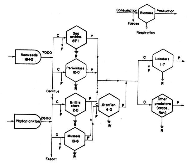
Figure 49 Energy flow through the sub-tidal benthic community in the seaweed zone of Saint Margaret's Bay, Nova Scotia. Units are Kcal/m2/year, except for biomass which is in Kcal/m2. Phytoplankton production figures are from Platt (1971) (After Miller, Mann and Scarratt, 1971)
Explanation to Figure 49: Figure 49 uses the energy-circuit language developed by H.T. Odum (see Platt, Mann and Ulanowicz, 1981 for details), where the seaweed bed is viewed as a combination of energy receptor (through photosynthesis) and self-generating consumer unit (by respiration): with a standing stock of 1840 Kcal/m2/yr, which contributes 7000 Kcal/m2/year to the population of herbivores and detritus feeders supported by it (each in turn representing a self-maintaining consumer population).
As shown in Figure 49, consumption of plant material produces faeces and detritus supporting benthos, and also shows a very significant net loss in the chemical energy content of food web constituents by respiration, as signified by the symbol indicating return to ground; (or to “sink” in the more usual energy circuit language).
The first important conclusion from this calculation is that annual seaweed production exceeds herbivore consumption by more than ten-fold: much of this material which is not consumed in situ, plus “secondary” detritus in the form of faecal material is exported from the local subsystem as broken pieces of fronds and other plant debris, and like other sources of detritus elsewhere, e.g., mangroves and seagrass beds, makes an important contribution to the food chains of adjacent shelf regions. This contribution has been estimated by Mann (1972) to be approximately equal to that from phytoplankton within the 90 m depth contour off Nova Scotia: illustrating its potential as a source of organic material for near-shore food webs.
Secondly, lobsters, starfish and other primary predators such as the wolf fish Anarhichas lupus control the population of herbivores, of which the most important is the sea urchin, Strongylocentrotus droehbachiensis, which is a major grazer of algae, and which in the 1960s showed major increases in abundance associated with a serious decline in kelp stocks. Absence of control of urchin populations due to overharvesting of primary predators was offered as the main reason for serious depletion of kelp beds in the 1970s from many apparently suitable rocky substrates along the Nova Scotia coast by Breen and Mann (1976) and Chapman (1981). In the 1970's it was also clear (Pringle et al, 1982), that overfishing as well as shortage of suitable habitat at key “bottle-necks” in the life history, rather than just limitations on food, were likely to be the responsible factors for the low population size of lobsters, and given the wide range of food accepted by lobsters, overfishing or loss of shelter may have been the most important effects.
In the light of extensive subsequent discussions held on the nature of the interaction described in the paper by Miller, Mann and Scarrat (1971), (see Pringle et al., 1982 for a review), it seems clear that although interesting, it is not evident here what the measurement of the energy flow in one or two limited locations has contributed to the resolution of the relative importance of the linkages described. This is partly because several essential pieces of information were missing at that time, related to the relative size and spatial interractions of the individual species components of the system, and not just their rates of feeding. It also is becoming clear that components not included in the preliminary energy-circuit diagram above may play an active part. This is also the case in the similar sea urchin - Macrocystis - Abalone - sea urchin - sea otter system referred to in Pringle et al. (1982), where the key role of other components (a sea star and labrid fish, not to mention the possible effects of coastal pollution), have all been considered as important factors in producing the community changes observed, in addition to the previously identified components mentioned above. It is clearly important to have some idea of the relative feeding rates and spatial overlaps of a given predator on one or other prey species.
The aspect that most occupied workers on this Nova Scotian system in the 1970s was the apparent irreversibility of the increase in urchin abundance, and the decline in kelp biomass, but as will be seen in the following, it is important to also be aware of the broader zoogeographical scale and longer term history of a system before drawing rapid conclusions. The above change to urchin dominance appeared irreversible because following active grazing down of mature kelp stands, urchins, although showing stunted growth, were able to persist and keep ‘barrens’ free of kelp sporlings while grazing on detritus material and other plant sporlings settling on the rock surface. At this point, Breen and Mann (1976) concluded from all available evidence, that it was “difficult to visualize a mechanism that would allow kelp beds to reappear”.
In 1980, such a mechanism made itself felt dramatically in the form of a sea urchin pathogen (Miller, 1985, 1985a), rather similar in its impact to that which in 1983 decimated populations of the tropical urchin Diadema antillarum throughout large areas of the Caribbean (Lessios, Glynn and Cubit, 1984). The Nova Scotian disease vector proved virulent and easily transmitted, and in two years (Miller, 1985, 1985a), some 250 000 t of sea urchins are estimated to have been killed. Kelp recovery rapidly followed, and the area of habitat now released to kelp production is estimated potentially to support a seaweed crop of some 1.8 million tons, and an annual production of some 7 million tons. It will be interesting to see what other ecological effects follows from this greatly increased production of coastal organic material; not only on the lobster stock, but on coastal production in general.
As a result of this experience, circumstantial evidence was collected that such urchin epidemics had occurred in the past, and Miller (1985) postulates a cyclical succession of fairly long period (Figure 50), with both urchin and kelp alternating in dominance.
The picture now seems a little clearer and more optimistic than in the 1970s for this system, though as in most ecosystem research, as many new questions are raised as were answered. For example, if the pathogen is so virulent, where did it come from? What will be the relative contribution of increased habitat versus food to coastal resources such as lobster that occupy the kelp zone? The one fact that cannot be doubted, is that ecosystem stability is less certain an axiom now than it seemed to be as little as 10 years ago.
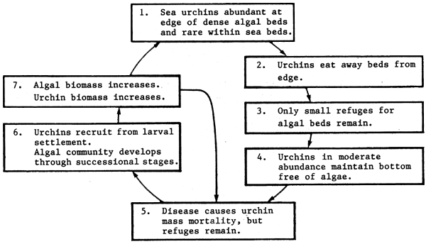
Figure 50 Seaweed-sea urchin cycle (from Miller, 1985a)
Seagrass nursery areas - juvenile and feeding habitats for many reef - dwelling species
Seagrass beds occur over a wide range of latitudes, from Tasmania to Japan and the Baltic Sea, (see review by Pollard, 1984), and in all areas play an important ecological role, which seems only in part to relate to their importance as a contributor to detritus food webs, especially leading to forage species of small epibenthic crustacea such as amphipods. These latter are important in the diets of early stages of juvenile fish; many of which use seagrass beds as shelter from predators. This habitat thus provides shelter to juveniles of fish species and lobsters, and is a foraging area for predatory and herbivorous species, especially in the tropics from adjacent coral reef areas. These feed over seagrass beds, often on a nocturnal cycle: returning to the reef areas during the day. This observation suggests care should be taken in assuming that the very high production estimates observed in some coral reef areas are entirely due to primary production from reef areas alone.
There seems to be some question in the literature as to how much of the seagrass production results directly from its grazing by herbivores: like other macroscopic plants we have mentioned, much of this plant production seems to enter the food web through detritus: especially through the crustacean linkages to juvenile fish. The high figures for fish production of seagrass beds apparently results from the large number of young of the year which are growing at very high rates (Thayer, Adams and La Croix, 1975).
One other feature of this and other types of marine vegetation (as well as other types of outcrops from the sea floor), is the high surface area they provide for larvae settlement, and for epifauna and flora: this perhaps is of comparable importance ecologically to the direct contribution of seagrasses to herbivore food chains, and this aspect of extensive substrate surface and shelter from predators must be a common feature of many fish nursery areas. In the case of seagrass, it may be that a change in the fractal nature of the habitat makes it a less secure shelter for organisms over a certain size: the size at which many juvenile fish move to other habitats. Also, despite their importance at key juvenile stages, it has been noted that grass beds, with some exceptions, are relatively less important as fish spawning areas.
The growing understanding of the significance of such centres of primary production in the nearshore and littoral zone, and the potential impacts of a variety of human activities (e.g., dredging, mine runoffs, urban wastes, etc.) on these habitats, constitutes one area in which an application of the constraints of marine ecology contributes directly to maintenance of healthy levels of near - shore fish production.
Experimental work is now beginning to accumulate on the possibility of restoring depleted seagrass beds (e.g., Thorhaug, 1985), following large scale interventions in near shore ecosystems.
An example of the construction and potential use of qualitative food web concepts in fisheries management is the demersal fish community of the shelf and slope of the Baleares and Western Mediterranean: a fauna that is intermediate in complexity between relatively species - poor areas such as the northwest Atlantic and upwelling areas of the world, and the much more complex and diverse fish communities of tropical areas. A matrix of the trophic inter - relationships of this fish community is shown in Macpherson (1981), who also describes some of the important benthic and planktonic invertebrates in the food web. These lower components of the three “trophic levels” shown in Figure 51 are given an arbitrary trophic number, beginning with those fish species - the inner circle - which are exclusively invertebrate feeders. Interestingly enough, Molva is the only fish species here in which invertebrates do not play any significant role in the diet. Although they are not shown here, it should not be forgotten that invertebrates themselves do not occupy a single trophic level, and that even among invertebrate feeding fish, a considerable degree of resource partitioning occurs (MacPherson, 1981).
Trophic classification and the compartment model approach to representing trophic interrelationships
One alternative approach that summarizes the whole of Table 1 in Macpherson (1981) is shown in Figure 52, which is essentially a compartment model indicating where the energy of the system comes from. This is instructive, from the structural point of view, in that two separate groups of “forage fish” may be recognized in the two large basal circles, largely feeding on planktonic and benthic food respectively; (although here a degree of overlap certainly occurs: nearly all benthic feeders must occasionally take some planktonic food, especially early in their life history, and possibly to a lesser extent, vice versa).
Considering the higher level predators, Figure 51 underlines the fact that for most of them, invertebrates still make up a significant part of their diet. Despite this, three basic predatory groups may be recognized:
Predators on largely planktivorous fish (Micromes and Scyliorhinus);
feeders on largely benthophagous fish (Phycis); and
mixed feeders, which consume most species.
From a research perspective, and bearing in mind what we have discussed earlier, some possible implications of this distinction that seem to merit further investigation are:
population sizes of category 1 species and their prey are a priori likely to be more volatile than category 2 species;
categories (1) or (2) species are less likely to be reciprocally affected by management measures on species in the other category, than species in the same category.
Other than this, we may consider compartment models as biologically interesting and useful in demonstrating how biomass or energy is partitioned, but if based on purely trophic criteria, of less immediate application to management of fisheries systems. Consequently we concentrate in this account on Figure 51) from now on, which describes individual species interractions.
The use of a circular format for the food web in Figures 51 and 53 is largely a graphical convention which stems from the need to maintain intelligibility by at least ensuring that crossover of linkages between components is minimized, and when it occurs, remains at as close to right angles as possible. Conceivably, it would have been more logical to have reserved the inner circle for the apical predators (see, for example, Figure 53), but since the commercial emphasis is on those economically more important species generally higher in the food web, which are here shown with larger circles, the present arrangement has some underlying logic, as well as conveying the basic idea of dissipation of benthic productivity upwards through the food web, rather than production being targeted toward a single apical predator, which is evidently not the case here.
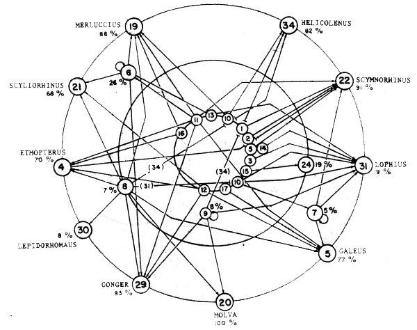
Figure 51 Showing detailed food web linkages for a Mediterranean demersal fin-fish community after MacPherson (1981). The “apical” predators are shown in the outer of the three concentric circles, and “forage” fish (purely invertebrate feeders) in the inner circles. Percent points by each component indicate percent of fish in the diet. Components (e.g., Nos. 6, 7 and 9), with self - directed arrows, are in part cannibalistic
Although the concentric circles in Figure 51 do not accurately represent trophic levels, the convention is adopted of showing cannibalistic species half a “trophic level” higher than otherwise, on the grounds that they share some of the characteristics of their predators. Thus Antonogadus (species no. 9) is exclusively invertebrate feeding, except for a predeliction for consuming its own kind, and is shown half - way between the first and second levels. Similarly this applies for Micromesistius (6) and Phyics (7); cannibalistic species which also consume other fish species as well as invertebrates. It may or may not be a coincidence that with species (8), these cannibalistic species (Micromesistius pontassou), Phycis blennoides and Antonogadus megalokynodon) play a key role in the diets of the apical predators, and we can speculate (Ursin, 1982) that they may be able to move upwards in the heirarchy to occupy the place of one or more of the apical predators should they be temporarily reduced in numbers.
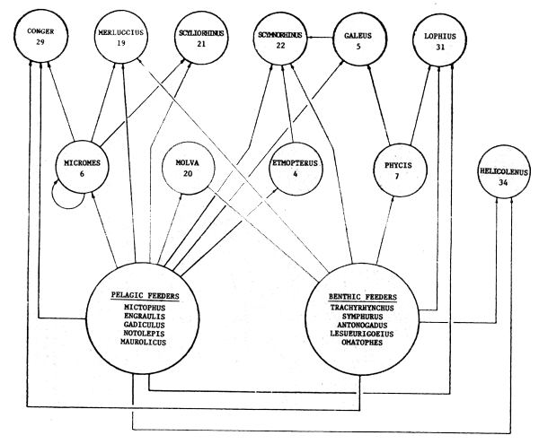
Figure 52 Compartment model for the same system shown in Figure 51, illustrating the two main groups of forage fish, classified by their predominant food type
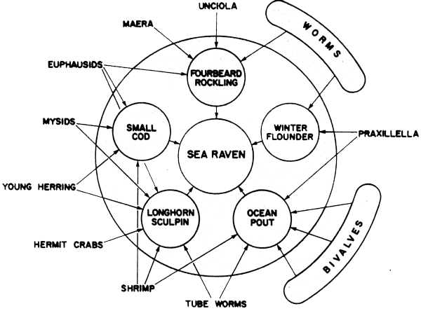
Figure 53 Showing the “Energy usage group” of the sea raven (Hemitripterus americanus): (in contrast to Figure 43, forage species are shown outside the outer circle) (From Tyler, Gabriel and Overholtz, 1982)
Several features of this food web attract our attention and may have significance:
Discounting the fragile distinction that a few species (nos. 6,7,8,9 and 24) are only one linkage at maximum above the level of wholly invertebrate feeders (invertebrates in fact make up a large part of their diet), there is no real distinction between arbitrary levels 2 and 3. In fact, for the most part (except Molva), invertebrates play an important part in the diet of all components, so that ‘percent invertebrates’ in stomach contents might be inversely related to ‘height’ in the food web, and as such used as a rough index of trophic level.
Also more or less as a consequence of (1), we may consider this food web as essentially very broad and shallow. Although some higher components may exist that are not shown (e.g., sharks), there appear to be few if any components wholly dependent on a single item in the diet.
One of the other interesting features of this food web is the relatively infrequent occurrence of cannibalism (which can be regarded either as an intraspecific population control device, or as a mechanism for population survival in limiting food conditions -see later), and the apparent absence of reciprocal predation. This last phenomenon (mentioned earlier between herring and cod) would undoubtedly be seen if larval stages were considered, but seems to be absent in the macrofaunal fish components. The explanation for this appears to be that individual size ranges of species as adults are relatively limited (compared to high - latitude commercial species) and stratification by size in this community is rather well developed with many small species, and a relatively large ratio of mouth gape to body size for the fish predators. It would be interesting to know to what extent this is true of tropical fish communities: certainly the ratio mouth gape/body length should be some measure of the degree of “compression” of the food web into a given total range of sizes in the ecosystem. An example of the wide range of this ratio in nature has already been given in Figure 10B. (Note, however, the importance of effective gill raker spacing in facultative particle feeders, e.g., many scombrids).
There is a large degree of overlap between the diets of the apical predators, suggesting that the system should accommodate to a moderate intensity of fishing effort on any one predator species, i.e., there should be a relatively low probability of population explosions or catastrophes in population size of prey species as a result of reducing the abundance of any one predator in the system. This speculation is of interest in view of the major local historical fluctuations shown by catches of one of the more important predators, the hake Merluccius. We may question whether the other predators sharing in part the same prey showed population increase out of phase with hake or alternatively, whether fluctuations in the prey species were the main casual agent for the fluctuations. An investigation of these relative abundance changes with time will be very instructive in this regard. The following subset of the above food web may then have management implications:
PREDATORS:
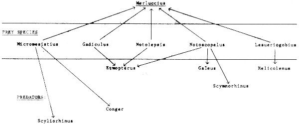
Two types of interaction may be detected between the key commercial species Merluccius and other components of the system: competition between predators, and mutual impacts of predator and prey populations. Simple measures of these two potential impacts are given in the following table, namely, the percent similarity of the diets (effectively the percentage of diet in common between two predators), and the combination of availability and “preference” (as judged by the ranked percent of a given prey species in the stomachs of hake and the other predators). Both of these criteria may be used to determine whether changes in hake population size are likely to have an impact on other directly - linked food web components.
| Ranked similarity of diet with Merluccius (%) | Ranking by importance of Merluccius as a predator in terms of the proportion of prey in stomach contents | |||
|---|---|---|---|---|
| 1 | Scyliorhinus | 35.4 | Lesueriogobius | 1 |
| 2 | Etmopterus | 33.0 | Micromesistius | 2 |
| 3 | onger | 26.5 | Notolepis | 2 |
| 4 | Galeus | 10.3 | Notoscopelus | 6 |
| 5 | Helicolenus | 10.1 | Gadiculus | 9 |
| 6 | Scymnorhinus | 4.8 | ||
Several other simple indices may be proposed, in particular, the relative consumption of a given prey by a given predator. This could be most easily measured by:
(% wt. of a given prey in the stomach) x No. (wt.) of predators.
This index should preferably also be adjusted by the rate of food consumption of the predator before comparing between species, and also ideally take into account the seasonally - adjusted percent habitat overlap of the predator and prey. In conclusion, an index of competition (Ic) between predators A + B could be postulated:

and an index of potential impact (IP) of predator C on prey D by:

Comparison of the components of a food web in this fashion might detect pairs of species most likely to be affected by changes in biomass of the other. This should be helpful in preliminary risk evaluation of possible effects of intensive harvesting of one or more species on others of similar diet, or which are key predators or key dietary items for the species in question.
Ecosystems in upwelling areas
In general, Mediterranean demersal food chains such as we have just been discussing, are nutrient limited, and usually have a rather high diversity with a wide range of species sharing the biomass.
In contrast to this type of habitat we may consider the ecosystems of upwelling areas: (see Sharp and Csirke, 1983; Bas, Margalef and Rubies, 1985) for more details on these systems). Upwelling areas support some of the world's most productive fisheries. Even in low latitudes, such systems are driven by cold nutrient - rich water rising to the surface as a result of hydrodynamic forces, principally the effects of offshore winds, which are often seasonal in occurrence, as is the upwelling ‘event’ in most cases. Typically, the strength of upwelling varies from year to year (Figure 54), and the fish catch with it (Figure 55): making these areas very dependent on environmental factors as well as on fishing effort, for short-medium term fish production.
In contrast to other high diversity, nutrient - limited habitats such as those typical of coral reef areas in the tropics, areas of upwelling are nutrient-rich, and support a high production of phytoplankton leading to shallow food webs showing a high species dominance by relatively few resident components. Each component is characterized by a high biomass which is rather variable in time. In some respects, as noted by Cushing (1982), these systems show a similarity to the fisheries of productive high latitude areas, such as the North Sea, with certain obvious substitutions, in that the “cods” are often replaced by hakes, the mackerel by jack mackerels, and the herrings and sprats by sardine and anchovy: this is obviously a gross oversimplification, in that some groups such as the hakes also occur outside upwelling systems, while important components for example, the cephalopods and sparids are not mentioned. For most upwelling systems, this similarity is nonetheless reinforced by a seasonality of production, which also contributes to the generally low stability and diversity of such systems.
Ryther (1969) notes that the average length of food chains is shorter in oceanic upwelling areas, and this is related directly to a low diversity and an earlier successional stage than more stable systems elsewhere. Much of the production is transported away from the immediate centre of upwelling; both horizontally, to adjacent areas (Figure 56); and vertically, with depth to benthic food chains (Figure 4). Thus, it has been noted that lower trophic levels in upwelling areas are often displaced in space with respect to one another, progressively away from the centre of upwelling. Thus, off the coast of NW Africa for example, primary production is not intense close to the coast, but the greatest zooplankton production is near the edge of the shelf. For fishes and other predators higher in the food chain of seasonal upwellings (e.g., Figure 21), a degree of seasonal mobility or migration is called for, which may take them still further from the centre of production. Transportation may be passive: cold, upwelled water can be carried for at least 100 km from the point of emergence; thus forming what we have referred to as a dissipation structure (Figure 56), in which the centre of production of successively higher elements in the food webs are displaced laterally (by drift and migration) from the centre of primary production. Jones (1982) notes that the importance of this surface residence time is that primary production can be completed and assimilated into the trophic chain before the cold water sinks again: thus accounting for the short food chains. By lateral advection, however, the impact of upwelling systems may extend to a considerable distance from this centre, both because of ‘leakage’ of nutrients horizontally and precipitation of detritus vertically. As noted, “leakage” occurs also through the seasonal migrations of many fish species, which dissipate nutrients from centres of high production. Migration is also necessitated by phenomena associated with seasonal upwellings, such as the tipping of oxyclines and thermoclines, which can result in low oxygen bottom water approaching the surface and making such waters uninhabitable for many species. Leakage occurs vertically also to the benthic systems, which may show a tendancy toward anoxic conditions due to decomposition of abundant detrital “rain” from the pelagic production system.
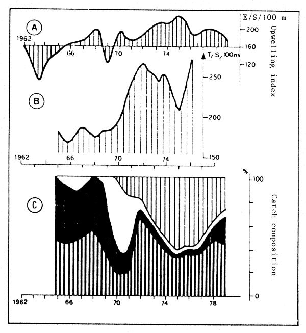
Figure 54 (A) Variations in upwelling strength in the central part of the CECAF area
(B) Variations in upwelling of catches southern area
(C) Changes in species composition of catches
(From Gulland and Garcia, 1984)
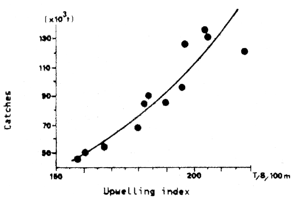
Figure 55 Relationship between annual catches and upwelling in the CECAF area (From Gulland and Garcia, 1984)
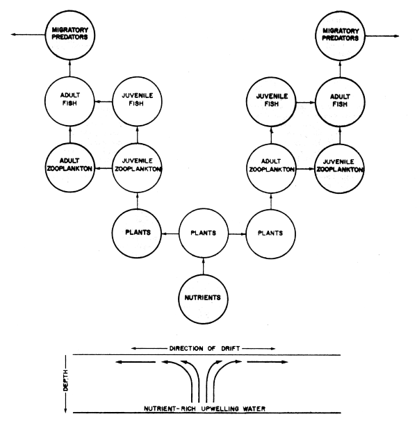
Figure 56 Dissipation structure typical of food webs of upwelling areas (Modified after Jones, 1982)
It follows from the generally low diversity of upwelling ecosystems that food webs are simple and that the size spectrum of organisms at any one time is likely to be somewhat discontinuous. Despite high food abundance, this could lead to problems in locating appropriate sized food particles at key stages in the life history of resident species, since size preferences of food necessarily change as a species completes its ontogeny.
One consequence of this may be the fact that several key components of low diversity environments show cannibalistic features in their life histories, e.g., squids (Amaratunga, 1983), anchoveta (Santander, 1981) and hakes (Lleonart, Salet and MacPherson, 1983): the young of the year of Merluccius (and the smaller individuals of a cohort (males), in the case of Illex), providing a “safety net” for diets of mature females, thus aiding production of a second generation under otherwise uncertain trophic conditions. Such mechanisms also would serve as density dependent population control mechanisms; “damping out” wide fluctuation in abundance in relatively simple food webs. (See Figure 57 for a rather speculative view of such a triangular component in upwelling food webs).
Csirke (1980) described how anchovy recruitment is a function of two processes: a stock dependent mechanism where egg production decreases at high population levels, and a density dependent mechanism where prerecruit survival is a function of year class size and environmental events. These year to year events include the variable degree of development of the El Niño (upwelling) phenomenon, which in turn, has a controlling influence on dominance among anchoveta and sardine (Santander, 1981): the former being associated with the high production areas close to the upwelling, the latter being more dominant in less productive oceanic water farther from the coast. In years of less intense upwelling, these species ranges become more closely coincident, and direct competition of larvae, as well as the high densities of spawning anchoveta close to the coast, must also result in high levels of cannibalism of anchoveta eggs at this time (see Csirke 1980; Sharp and Csirke, 1983 for further discussion).