7.1 Profit of
a Business
7.2 Cash Flow Diagrams
7.3 Methods of Estimating Profitability
7.3.1 Rate of return
7.3.2 Present worth (PNV)
7.3.3 Discounted cash flow rate of return (DCFRR)
7.3.4 Pay out time
7.4 Risk
Consideration
7.5
Advantages and Disadvantages of the Different Methods of
Estimating Profitability
7.6 Break-even Analysis
7.7
Profitability of Artisanal Fisheries
7.8
Profitability for Small and Medium Fish Plants
7.9
Inflation in Profitability Calculation
7.9.1 Effect of inflation on the present-worth (PW)
7.9.2 Effect of inflation on the IRR. Real Internal Rate of Return
7.9.3 Effect of the adjustment of working capital on the IRR
7.9.4 Inflation relationships in continuous form
7.9.5 Effect of financing of working capital on the IRR
7.9.6 Effect of loans on the investment on the IRR
7.9.7 Effect of the non-indexed loans on the investment on the IRR
7.9.8 General conclusions on inflationary situations
"Profitability" is a general term which measures the income that can be earned in a particular situation. It is the common factor in all productive activities. Some parameters need to be introduced in order to define profit. Gross profit (GP) for the company equals the income from total sales (S) less total production costs without depreciation (C), as follows:
GP = S-C (7.1)
When considering depreciation costs, net profit before taxes (NPBT) results:
NPBT = GP - e x IF = S - C - e x IF (7.2)
where: e = internal depreciation factor.
Taxes are imposed on these gross earnings such that the investor does not receive the entire sum of money. They constitute an important factor in evaluating the economy of alternative courses of action. The level of taxation differs in each country, for example (French Institute of Petroleum, 198l):
Country Percentage USA 52 Canada 41 Germany 51 France 50 Italy 35 UK 53.75 Japan 50
For example, the rate of taxation in 1980, in USA, was applied in the following way (Jelen and Black, 1983):
| Percentage | |
| Rate on the first US$ 25 000 earned: | 17 |
| Rate on the next US$ 25 000 earned: | 20 |
| Rate on the next US$ 25 000 earned: | 30 |
| Rate on the next US$ 25 000 earned: | 40 |
| Rate on earnings above US$ 100 000: | 46 |
The same type of situation can be found in developing countries. For instance, in 1969, the following taxation scale was used in Peru (Engstrom, et al., 1974):
| Percentage | |
| For income under US$ 2 326 | 20 |
| Income between US$ 2 326 and 11 628 | 30 |
| Income above US$ 11 628 | 35 |
It is noted that taxation levels and procedures change in some countries frequently (e.g., yearly). When it is not possible to determine the actual tax, an arbitrary tax of 40-50% of net profit before taxes is suggested. Net Profit (NP) can be calculated as follows:
NP = S - C - e x IF- t (S - C- d x IF ) (7.3)
where: d = official depreciation factor and t = taxation rate.
The passage of money into or out of the enterprise is called cash flow and is defined as the difference between income and operating costs, excluding depreciation and after payment of taxes; it can be expressed as follows:
CF = NP + e x IF = S - C - t x (S - C - d x IF) = GP - t x (S-C-d x IF ) (7.4)
Cash flow or net profit is not a measure of profitability but these figures are used to calculate profitability of a particular project. The aim of an investor or company is always to maximize earnings with respect to the costs of the capital to be invested. If the aim were solely to maximize earnings, any investment that might yield profits would be acceptable, despite low returns or high costs.
In economic studies where different alternatives for a project have to be compared, or a comparison made between the profitability of a project and the profitability of existing financial transactions, methods of analysis are used that will allow this estimate to be made on a uniform basis.
All investment projects indicate an action that will develop over a number of years in the future. The study of the financial characteristics of a project requires analysis of the time value of money, financial risk, future variations in sale prices, costs, volume of sales and taxation rate, and the time needed to implement the project or install the equipment before starting normal production and the economic life of the project. Such factors are the following:
IF = Depreciable Original Fixed Investment
Iw = Working Capital
IR = Residual Investment = Land + Iw
A = Annual Earnings
B = Annual Cash Generation from Depreciation
C = Construction Period
A way of visualizing many of these factors is to use a cash flow diagram like that shown in Figure 7.1 (Perry and Chilton, 1973).
In Figure 7. 1, money is shown on the y-axis and time on the x-axis. Zero time is the point at which the plant begins to produce. In negative situations, the only cash flow is negative, as this is the money paid for land and fixed investment, IF . When the process is ready to begin, there is an additional quantity of money to consider within working capital Iw. When the process begins production, the money enters the project as a product of sales: S. The cash flow accumulates, moving from negative to positive, and when the project ends, the capital invested in current assets and land is recovered, resulting in a positive final cash flow.
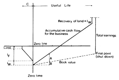
Figure 7.1 Cumulative Cash Flow for a Project
This diagram has the advantage of showing all financial characteristics, with the except for risk, the rate at which the project generates money and the earnings for reinvestment.
Financial plans can be simply presented by integrating all data into "statements of sources and application of funds". These statements show the origin or source of the funds and their final destination.
Example 7.1 Statements of Sources and Application of Funds
Prepare a statement on the sources and application of funds for the frozen hake plant in Example 2. 1.
Data:
IF = US$ 600 000 (from Example 3. 1)
Iw = US$ 60 000 (from Example 3. 1)
Daily Production = 2 t FB
Working days of the year = 270
N = 10 years
Selling price = US$ 1 560/t FB
Unit Production cost = US$ 1 272 /t FB (Example 4.4)
Answer:
Annual sales = Annual Production (t FB/year) x Selling Price (US$/t FB) = 2 t FB/day x 270 days/year x 1 560 US$/t FB = 540 t FB/year x 1 560 US$/t FB = 842 400 US$/year
Annual production cost = Annual production (t FB/year) x Unit production cost (US$/t FB) = = 540 t FB/year x 1 272 US$/t FB = 686 880 US$/t FB
The straight-line method of depreciation is used. The results are given in Table 7. 1.
Table 7.1 Statement of Sources and Application of Funds for a Fish Plant (in US$ '000)
Activity |
1990 |
1991 |
1992 |
1993 |
1994 |
1995 |
1996 |
1997 |
1998 |
1999 |
Source |
||||||||||
Own capital |
480 |
|||||||||
Bank credit (*) |
180 |
|||||||||
Net sales from activity |
842 |
842 |
842 |
842 |
842 |
842 |
842 |
842 |
842 |
842 |
Total (a) |
1502 |
842 |
842 |
842 |
842 |
842 |
842 |
842 |
842 |
842 |
Applications |
||||||||||
Fixed investment |
600 |
|||||||||
Working capital |
60 |
|||||||||
Costs of financing (**) |
27 |
|||||||||
Costs of production |
687 |
687 |
687 |
687 |
687 |
687 |
687 |
687 |
687 |
687 |
Total (b) |
1 374 |
687 |
687 |
687 |
687 |
687 |
687 |
687 |
687 |
687 |
(a) - (b) |
129 |
156 |
156 |
156 |
156 |
156 |
156 |
156 |
156 |
156 |
| Net profit (***) | 77 |
93 |
93 |
93 |
93 |
93 |
93 |
93 |
93 |
93 |
Plus depreciation |
60 |
60 |
60 |
60 |
60 |
60 |
60 |
60 |
60 |
60 |
Cash flow |
137 |
153 |
153 |
153 |
153 |
153 |
153 |
153 |
153 |
153 |
Notes:
(*) There is a bank credit, 30% IF=US$ 180 000.
(**) Bank rate on loan 15% per year. For simplicity, only a one year credit has been considered.
(***) Taxes to be deducted from earnings (40%).
The most common methods of evaluating profitability are the following:
Rate of return on the original investment (iROI)
Rate of return on average investment (iRAI).
Present-worth (PW)
Internal rate of return (r)
Pay out time (nR)
In economic engineering studies, the rate of return on investment is normally expressed as a percentage. The annual net profit divided by total initial investment represents the fraction which, when multiplied by 100, is known as the percentage return on investment. The usual procedure is to find the return on total original investment, with the value of the average net profit being the numerator:
(7.5)
and thus, the rate of return on the original investment, iROI, will be:
(7.6)
Due to the depreciation of the equipment during its useful life, it is usual to relate the rate of return to the average investment estimated during the useful life of the project. Average investment (lj is found as follows:
(7.7)
where Bk = Book value in year k.
It can also be used an approximate formula to calculate the average investment:
Ia = IF / 2 (7.8)
The rate of return on the average investment (i RAI) can be determined by the following equation:
(7.9)
The method to calculate the rate of return on the original investment (i ROI) is also known as the engineering method, while the method that calculates the rate of return on the average investment (i RAI ) is the method preferred by accountants.
These methods give "point values" which are applicable in a particular year or for some "average" year chosen. No account is taken of inflation, or of the time value of money.
Example 7.2 Calculation of Rate of Return on Original Investment (i ROI)
Calculate the rate of return on original investment for the frozen hake plant in Example 7. 1.
Answer: In this case where the annual cash flows are not constant, the following must be calculated:
Average annual net profit = Annual cash flow - Annual depreciation costs (7.10)
The resulting values are shown in Table 7.2
Table 7.2 Calculation of Average Annual Net Profit for the Plant in Table 7.1
Year |
Average Annual Profit (US$) |
1 |
77000 |
2 |
93000 |
3 |
93000 |
4 |
93000 |
5 |
93000 |
6 |
93000 |
7 |
93000 |
8 |
93000 |
9 |
93000 |
10 |
93000 |
Total |
91400 / 10 = 9 140 |
The average rate of return on the original investment will be:
(9 140 ÷ 660 000) x 100 = 13.8% per year
The time value of money is not considered, since only the average profit is used, not its timing. The profits from years 1 through 10 could be reversed and the return on original investment would be the same.
Example 7.3Calculation of Rate of Return on Average Investment (i RAI )
Calculate the rate of return on average investment for the frozen hake plant in Example 7. 1.
Answer: In order to correctly determine the average investment, the average investment must be calculated according to Table 7.3.
Table 7.3 Calculation of Average Investment for the Plant in Table 7.1
Year |
Investment (US$) |
1 |
600 000 |
2 |
600 000 - 60 000 = 540 000 |
3 |
546 000 - 60 000 = 480 000 |
4 |
492 000 - 60 000 = 420 000 |
5 |
420 000 - 60 000 = 360 000 |
6 |
360 000 - 60 000 = 300 000 |
7 |
300 000 - 60 000 = 240 000 |
8 |
240 000 - 60 000 = 180000 |
9 |
180 000 - 60 000 = 120000 |
10 |
1120 000 - 60 000 = 60000 |
Total |
3300 000÷10 = 330 000 |
From Table 7.3., the divisor of Equation (7.9) is:
Ia + Iw = US$ 330 000 + US$ 60 000 = US$ 390 000
and the rate of return on average investment, will be:
91400 / 390 000 x 100 = 23.4% per year
Making an approximation with equation (7.8), it can be seen that:
91 400 x 100 / ((600 000 / 2) + 60 000) = 25.4 %
which shows a 8.5 % error in the estimate. The time value of money is not considered, since only the average investment is used, not its timing.
This method compares the present-worth (PW) of all the cash flows with the original investment. It assumes equal opportunities for re-investment of the cash flows at a pre-assigned interest rate. This rate can be taken as the average value of the rate of return on the capital of the company or designated as the minimum return acceptable for the project. The procedure followed compares the magnitude of present-worth of all revenues with investment at time 0. The net present value is a single amount referred to zero time and represents a premium if positive, or a deficiency if negative, at a chosen fixed rate of return.
(7.11)
Present-worth can also be defined as the additional amount that will be required at the beginning of the project, at a pre-assigned interest rate, to produce income equal to, and at the same time as, the prospective investment. Results do not indicate the magnitude of project. For that reason, the ratio of the discounted cash flow to investment is also suggested as a criterion (Equation 7.12)
(7.12)
This relationship can be used as an indicator of the profitability of the project by analysing the difference between the result and the unit value. The unit will be found where the pre-determined rate coincides with the value of the internal rate of return (see section 7.3.3). The results from both calculations (Equations 7. 11 and 7.12) can give some idea of the total magnitude of the project.
Example 7.4 Calculation of Present-worth
Calculate: (a) the present-worth (M) and (b) the PW' relationship for the frozen hake plant in Example 7. 1.
Answer: Applying a rate of i = 15 % per year in Equation (7. 11), the following results are obtained:
It should be noted that the salvage value and working capital must be included with the last year cash flow.
(a) PW = US$ 770 182 - US$ 660 000 = US$ 110 182
At the end of ten years, the cash flow to the project, compounded on the basis of end-of-year income, will be:
F = 137 000 x (1.15)9 + 153 000 x (1.15)8 + 153 000 x (1. 15)7 + 153 000 x (1.15)6 + 153 000 x (1.15)5 + 153 000 x (1.15)4 + 153 000 x (1.15)3 + 153 000 x (1.15)2 + 153 000 x (1. 15) + 213000 = US$ 3 115 816
This amount represents the future worth of the proceeds to the project and must equal the future worth of the initial investment plus the present-worth compounded at an interest rate of 15 % per year.
F = (660 000 + 110 182) x (1.15)10 = US$ 3 115 816
Thus, when US$ 110 182 is added to the investment (US$ 660 000) the result will be the sum that should be invested, at 15%, to generate annual income equal to, and at the same time as that estimated by the recommended investment.
(b) The relationship between the present-worth of the annual cash flow and the total investment, from Equation (7.12):
PW' = 770 182 / 660 000 = 1.17
This method takes into account the interest on the money invested, with time, and is based on the part of the investment that has not been recovered at the end of each year during the useful life of the project.
A trial and error method is used to establish the interest rate to be applied to the cash flow each year, such that. the original investment would be reduced to zero (or salvage value, plus land, plus working capital) during the useful life of the project.
In such a case, the resulting rate of return, is equivalent to the maximum interest rate that could be paid to obtain the necessary funds to finance the investment and completely paid back by the end of the useful life of the project.
Therefore, in this method, the present-worth of all cash flows is taken as zero and the internal rate of return, r, is calculated by trial and error:
DCFRR = IRR = r, where:
(7.13)
It should be noted that the application of computer technology to the preparation of feasibility estimates has become commonplace. Profit-estimating computer systems have a wide variety of applications, being used to increase accuracy and to reduce the time and cost of preparing capital-cost and profit estimates.
Example 7.5 Calculate the Internal Rate of Return (r)
Calculate the internal rate of return for the frozen hake plant in Example 7. 1.
Answer: At the end of 10 years, the present-worth of the cash flows (expressed dollars) will be:
(7.14)
which is equal to the present-worth of the initial, fixed investment, plus working capital.
PW = IF + Iw = US$ 660 000 (7.15)
An internal rate of return is obtained by making equation (7.14) equal to equation (7.15) and finding the value of r by trial and error. As mentioned before, this trial and error search can be done by computer, but in its absence, a discount factor is normally applied to the annual cash flows, in order to obtain the present-worth by applying various values of r, until the required value of the investment is obtained.
The discount factor for payments at the end of year M, is:
(7.16)
where:
r = selected interest rate
M = year for which the calculation is done.
Table 7.4 shows the trial and error method used in the example.
Table 7.4 Calculation of Internal Rate of Return for the Fish Plant in the Example 7.1
Trial for r = 0.1 |
Trial for r = 0.2 |
r = 0. 19 |
|||||
Year (m) |
Cash Flow (US$ '000) dm |
Factor |
Present-worth (US$'000) |
Factor dm |
Present-worth (US$'000) |
Factor dm |
Present-worth (US$ '000) |
0 |
(660) |
||||||
1 |
137 |
0.909 |
125 |
0.833 |
114 |
0.840 |
115 |
2 |
153 |
0.826 |
126 |
0.694 |
106 |
0.705 |
108 |
3 |
153 |
0.751 |
115 |
0.579 |
89 |
0.592 |
91 |
4 |
153 |
0.683 |
104 |
0.482 |
74 |
0.497 |
76 |
5 |
153 |
0.621 |
95 |
0.402 |
61 |
0.417 |
64 |
6 |
153 |
0.564 |
86 |
0.335 |
51 |
0.350 |
54 |
7 |
153 |
0.513 |
78 |
0.279 |
43 |
0.294 |
45 |
8 |
153 |
0.466 |
71 |
0.232 |
35 |
0.247 |
38 |
9 |
153 |
0.424 |
65 |
0.194 |
30 |
0.207 |
32 |
10 |
213 |
0.385 |
82 |
0.162 |
35 |
0.174 |
37 |
Total |
948 |
638 |
660 |
||||
Relationship = Total Present-worth / Original Investment |
1.44 |
0.97 |
1.00 |
||||
The interpolation to determine the correct value of r can be done by plotting the relationship between the original investment and the Total Present-worth as a function of r, as is shown in Figure 7.2.
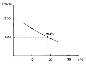
Figure 7.2 Interpolation for the Calculation of r, using the Values of Table 7.4
For simplicity, some columns for the dm factor have been omitted in Table 7.4 19. 1 % rate of return is the interest rate at which the original amount of US$ 660 000 be invested to generate income similar to, and at the same time as those calculated proposed investment. Thus,
660 000 x 1.19 = 785 697; 785 697 - 137000 = 648 697
648 697 x 1.19 = 772 241; 772 241 - 153000 = 619241
619 241 x 1.19 = 737 176; 737 176 - 153 000 = 584 176
584 176 x 1.19 = 695 432; 695 432 - 153 000 = 542 432
542 432 x 1.19 = 645 738; 645 738 - 153 000 = 492 738
492 738 x 1.19 = 586 580; 586 580 - 153 000 = 433580
433 580 x 1.19 = 516 156; 516 156- 153 000 = 363 156
363 156 x 1.19 = 432 319; 432 319 - 153 000 = 279 319
279 319 x 1.19 = 332 515; 332 515 - 153 000 = 179515
179 515 x 1.19 = 213 000; 213 000 - 213 000 = 0
It should be emphasized that the internal rate of return calculated for the plant in the example is lower than the rates observed for similar but larger plants. This result, in agreement with reality, is justified by the concepts discussed in Chapter 5.
Pay out time is defined as the minimum period of time theoretically necessary to recover the original investment in the form of cash flow from the project, based on total receipts less costs and excluding depreciation. Generally, the original investment only includes the initial, fixed, depreciable investment.
Pay out time, in years = Fixed Depreciable Investment / (average profit/year) + (average depreciationlyear) (7.17)
(7.18)
(7.19)
Example 7.6 Calculation of Pay out Time (nR)
Calculate the pay out time for the frozen hake plant in Example 7. 1.
Answer: The application of this method to the data in Table 7. l., gives the time required to reduce the investment to zero. From Equation (7.17):
nR = 600 000 / 151 400 = 3.96 years
which is an approximate value only coinciding with real value when cash flows are equal.
Table 7.5 shows that the investment will be reduced to zero between 4 and 5 years.
Table 7.5 Accumulated Cash Flow for the Plant in Table 7.1
Year |
Cash Flow (US$) |
Accumulated Cash Flow (US$) |
0 |
-600000 |
- 600000 |
1 |
137000 |
- 463000 |
2 |
153000 |
-310000 |
3 |
153000 |
- 157000 |
4 |
153000 |
- 4000 |
5 |
153000 |
149000 |
6 |
153000 |
302000 |
7 |
153000 |
455000 |
8 |
153000 |
608000 |
9 |
153000 |
761000 |
10 |
153000 |
914000 |
Values of Table 7.5 are plotted in Figure 7.3. This figure shows the graphical interpolation which gives a pay out time of 4.05 years. This is the real value of nR.
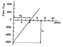
Figure 7.3 Graphical Interpolation for Obtaining Pay Out Time
Capital investments are made with the expectation of obtaining a substantial annual profit, but the possibility that losses might be incurred always exists. This factor, which accompanies all investments, is called "risk". In general, the greater the risk, the higher the expected rate of return and the shorter the time foreseen to recover of the investment.
Table 7.6, which gives average values for risk-free annual rates of return on capital investments for processing industries, allows comparisons to be made with the results of new feasibility studies on the expansion or modification of existing plants (Rudd and Watson, 1968; Woods, 1975).
Table 7.6 Average Profitability Values for Risk-Free Capital for Processing Industries
Industry |
Annual rate |
Public utilities (electricity and gas) |
6.3 |
Telephone companies |
6.8 |
Steel (USA) |
7.5 |
.General Motors |
7.8 |
Standard Oil |
8.2 |
Cellulose and paper, rubber |
8-10 |
Synthetic fibres, chemical and petroleum products |
11-13 |
Drugs and pharmaceutical products, extraction and mining industry |
16-18 |
From Equation (7.3), with d equal to e and constant, the Net Risk Profit (N-RP) is defined as:
NRP = (S-C-d x IF) x (1 - t) - iM x (IF + Iw) (7.20)
In Table 7.7, the minimum acceptable rate of profitability (iM) is shown as a function of the degree of risk (Happel and Jordan, 1981).
Table 7.7 Quantification of Risk
Type of Project |
Degree of Risk |
iM (%) |
Short project,
modification of existing plants |
low |
10-15 |
Specific equipment |
moderate |
15-25 |
Automatic
instrumentation |
high |
20-50 or more |
A result higher than zero indicates that the project has an annual profitability that exceeds the minimum acceptable rate, even when risk is taken into consideration. This method does not consider the temporal value of money, but more complete equations, such as the risk-value method, are given in the literature (Happel and Jordan, 1981).
Example 7.7 Calculation of Net Risk Profit (NRP)
Calculate the net risk profit for the frozen hake plant in Example 7. 1.
Answer: A minimum acceptable profitability rate of 10 % was selected from Table 7. 1. This is considered a low risk alternative. From Equation (7.20):
NRP = 91 400 - 0. 10 x 660 000 = US$ 25 400
A result greater than zero indicates that the project has an annual profitability that exceeds the minimum acceptable rate, even when risk is taken into consideration. It will be left to the reader to determine the profitability of the canning plant in Example 2.2, by using the same methods employed in Examples 7.1 to 7.7.
Data:
IF = US$ 130 000 (from Example 3.2)
Iw = US$ 13 000 (from Example 3.2)
Daily Production = 2 670 cans
Working days of the year = 250
n = 10 years
Selling price = US$ 0.8/can
Unit Production cost = US$ 0.68/can (Example 4.5)
Methods of return on fixed investment or on average investment give static values that can yield misleading results. These "point values" are either applicable for one particular year or for "average" years. Nevertheless, they are the easiest way to a quick estimate. Pay out time does not adequately account for the last years of useful life of the project. On the other hand, the internal rate of return method considers the time value of money and produces more realistic results than other methods. If there are investments after start-up time, the present-worth is the method that should be used, as the internal rate of return method gives multiple results.
What is the best profitability criterion? In practice, the analyst does not use a single criterion, but considers the use of various criteria to compensate for the advantages and disadvantages of each. Table 7.8 gives reasonable values for pay out time and internal rate of return for projects with different degrees of risk (Cunningham, 1980).
Table 7.8 Typical Values for Pay-out Time and Internal Rate of Return as a Function of Risk
Project |
Pay out time(years) |
Internal rate of return (%) |
High risk |
< 2 |
20 |
Normal |
< 5 |
15 |
Slight risk |
< 10 |
Key factors which affect profitability of operations in fish plants are generally cost and quality of raw material and the yield from processing, as long as the raw material is available and the market for the resulting products is stable (Montaner and Zugarramurdi, 1994).
Break-even analysis is a method of organizing and presenting some of the static, short-run economic relationships of a business. Economic production charts show how costs, sales, and profits will vary when the rate of production changes, other things being equal. These evaluations do not take into account the time value of money and data for decisions are believed to be acceptably accurate.
The best known break-even model relates fixed and variable costs to revenue for the purpose of profit planning. In general, the efficiency of production operations depends on the utilization of the plant. When the profit can be defined as a function of the level of production of the system, it is possible to select the level of production at which profits will be highest. Mathematically, calculations are:
Total Revenue = Selling Price (US$/unit) x Production Rate (unit/time) = P x Q (7.21)
Total Costs = Variable Cost (US$/unit) x Production Rate (unit/time) + TFC (US$/time) = V x Q + TFC (7.22)
Net profit before taxes = NPBT = Total Revenue - Total Costs = P x Q - ( V x Q + TFC) (7.23)
At the break-even point, profits equals zero and the output to break even can be calculated as follows:
Q = TFC / (P - V) (7.24)
The value Q indicates the volume at which revenue and total operating cost exactly break even. At this point, one additional unit made and sold would produce a profit. Until the breakpoint is attained, the producer operates at a loss. The effects of production rate and operating time on costs should be recognized. By considering sales demand along with the capacity and operating characteristics of the equipment, the analyst can recommend the production rates and operating schedules that will give the best economic results.
It is generally accepted that firms seek to maximize profit. The majority of microeconomic theories consider the firm as a profit maximizing entity. In the short-run during which output level can be varied but plant size cannot, the firm is faced with several alternatives of levels of production, each with different profits, so the alternative with the greatest expected earnings will be selected.
The quantity that the firm will produce depends on the characteristics of the market. In a perfectly competitive market, the equilibrium is reached at a total industry Output Of QT and at a price of P*. Each firm has a horizontal demand which intersects the vertical axis at the equilibrium price (P*). In this case, both marginal and average revenue are constant and P* = MR = AR.
All these relationships are shown in Figure 7.4.
Given that the firm can sell any quantity of product (Q) at the same price, its total revenue (TR) will be a line with a positive slope that begins at the origin. If the firm has a cost structure represented by the following curves: average total cost (ATC), marginal cost (MC), total fixed cost (TFC) and total cost (TC), what will be the total quantity (Q*) that the firm will decide to offer for sale, and what will be the profit in that case?
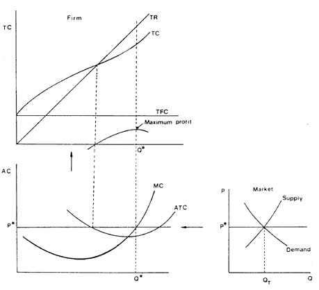
Figure 7.4 Equilibrium in the Short Run for a Firm Operating in a Perfectly Competitive Market
The response to these questions requires consideration of the aims of a firm producing in an environment of perfect competition: to maximize profits or to minimize losses. The easiest way of determining the point at which profits are maximized is to compare total revenue and total costs or to equal marginal revenue (MR) and marginal cost (MC). This rationale is shown in Figure 7.4. The firm maximizes profit by selling a quantity (Q*) for which MC = P*. The vertical distance between the total revenue line and the total cost curve indicates the profit. It will be maximum when Q* is the number of units produced. The firm's profit function is derived by subtracting TC from TR at each rate of output. In this system, it is also possible to incur losses in the short run and still continue producing, depending on the level of prices in the market and when this alternative will mean fewer losses than shutting down production entirely.
Figure 7.5. shows the case that a firm is facing by lower and lower P. Whether the firm realizes a profit or a loss depends on the relationship between price and average total cost at the intersection of MR and MC. The quantities to produce (Qd, Qc, Qb and Qa) for each different level of prices (Pd, Pc , Pb and Pa) are determined as: Price = Marginal Cost
The point (Qd, Pd) maximizes profit due to price Pd exceeds ATC.
The point (Qc, Pc ) a break-even point, profit equals zero. The price Pc, equals ATC.
The point (Qb, Pb) minimizes its short-term losses due to price Pb is less than ATC but higher than AW. So, the TFC are paid and the TVC are partially recovered.
The point (Qa,Pa) is a shutdown point, negative profit equals TFC or Pa = AVC.
Short-run losses equal to TFC will be incurred if production is temporarily ceased.
This conclusion is useful for deriving the supply curve for the firm in the short run (see Figure 7.5). Profit- maximizing firm's supply curve is its rising Marginal Cost curve.
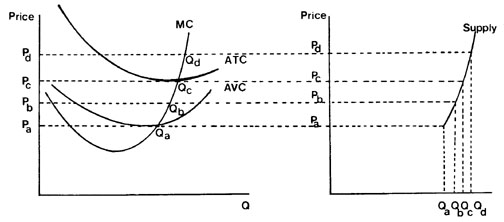
Figure 7.5 Supply Curve in the Short Run for a Firm Operating in a Perfectly Competitive Market
In the short run, a firm's capacity is limited by its fixed inputs, whereas in the long run, the options are numerous: its size can change, new technologies implemented, or the characteristics of its products can change according to changes in consumer tastes. As an extrapolation of these concepts, each business can determine its supply curve in the long run. In reality variations do occur, depending on the structure of the competition; that is, whether there are few or many suppliers or depending on whether the products are identical or varied. Four types of market structure can be identified:
Perfect Competition : many sellers of a standardized product
Monopolistic Competition : Many sellers of a varied product
Oligopoly Few sellers of a standard or varied product
Monopoly Single seller of a product for which there is no substitute.
Example 7.8 Determination of the Break-even Point for a Frozen Fish Plant
Analyse the frozen hake plant in Example 2. 1. Plot the total costs, variable costs, fixed cost and income from sales curves on a graph and determine the break-even point.
Answer: Data:
Selling price US$ 1 560/t of frozen fillet blocks
Unit Production cost = US$ 1 272/t FB (Example 4.4)
Unit Variable cost = US$ 1 085.5A FB (Example 4.4)
Unit fixed cost = US$ 186.5/t FB (Example 4.4)
Daily Capacity = 2 t FB
Working days of the year = 270
Equation (7.21) and (7.22) are applied to calculate TR, TVC, TFC, TC and NPBT over the range from 0 to 100% capacity.
Annual revenue = US$ 1 560/t FB x Q (t FB/year) = 1560 x US$ Q/year
Annual production cost =
= US$ 1 085.5/t FB x Q (t FB/year) + US$ 186.5/t FB x 540 t FB/year =
= US$ (1 085.5 x Q + 100 710)/year
From Equation (7.24), the break-even point can be calculated as:
N = 100 710/(1 560 - 1 085.5) = 210 t FB/year
Table 7.9 and Figure 7.6 show the variation of the different parameters.
Table 7.9 Revenue, Cost and Profit for Different Levels of Production for a Frozen Hake Plant
Percent utilization |
Q (t/year) |
TR (US$ '000) |
TVC (US$ '000) |
TFC (US$ '000) |
TC (US$ '000) |
NPBT (US$ '000) |
0 |
0 |
0 |
0 |
100.71 |
100.71 |
-100.71 |
20 |
108 |
168.48 |
117.23 |
100.71 |
217.94 |
-49.46 |
40 |
216 |
336.96 |
234.47 |
100.71 |
335.18 |
1.78 |
60 |
324 |
505.44 |
351.70 |
100.71 |
452.41 |
53.03 |
80 |
432 |
673.92 |
468.94 |
100.71 |
569.65 |
104.27 |
100 |
540 |
842.40 |
586.17 |
100.71 |
686.88 |
155.52 |
Figure 7.6 illustrates the relationship between fixed cost and total cost and level of output, as well as income and level of output.
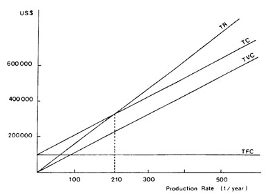
Figure 7.6 Graphical Representation of Break-even Point for a Frozen Hake Plant
For a linear break-even chart, profitable operation occurs to the right of the breakeven point (39% of utilization of the plant or 210 t FB per year or 0.78 t FB per day). If production is lower, the operation will incur losses. If production is higher, earnings will be obtained.
Example 7.9 Determination of Break-even Point for a Fishmeal Plant
Analyse the break-even point for the fishmeal plant in Example 5.3, which processes 500 t of raw material daily.
Answer: Figure 7.7 shows the break-even point graph for the values given in Table 5.6, for the 500 t/day plant.
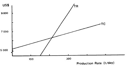
Figure 7.7 Break-even Point Graph for a 500 t of Raw Material per day Fishmeal Plant
In artisanal fisheries which exploit a great number of species, prices are frequently fixed by or for different species of equal size. These groups may or may not have similar biological characteristics. For the commercial species, the price is set in a manner directly proportional to the consumer's preference. Although they can change substantially during certain seasons, due to variations in the volume caught, variety of species and during cultural and religious events, these prices are generally stable. As a result, there is a difference in income received by each business in the course of any given year (Stevenson et al., 1982).
To improve the economic balance, countries support small-scale fisheries with different methods of financing. For example, in Ghana and Senegal, the Government has implemented a system which focuses mainly on the reduction of duties on fuel which have been used by fishing vessels and canoes for more than 10 years. This policy of reducing operational costs has a favourable influence on motorization in both countries. In Ghana, prices have been reduced from US$ 0.80 to US$ 0.25 per litre, while in Senegal it is less than half the regular price of US$ 0.50 per litre.
At times this type of policy can result in distortions, as engines that are larger than necessary are bought, and movable rather than stationary winches are used which increase the operational costs of the sector and the economy in general (Greboval, 1989).
Another study conducted in Seychelles (Parker, 1989) showed that if economic difficulties are experienced by small fishing vessels, those craft between 8 and 13 m long also suffer, due to the greater quantity of capital invested in each fishing unit. For this reason, the economic yield of three units of this type of fishing vessel is analysed:
Standard model (with 27-37 hp engine)
Standard model with echo-sounder and electric reels (chosen because a better catch was obtained), 56 hp engine
Similar to second model, with equal capacity, but with 70 hp engine (11.6 m long)
Income from a single trip can be considered as a function of the prices, rate of capture attained by types of fishing gear used, composition of catch and duration of trip (limited to the capacity to maintain the vessel). In the first instance, the estimated income per trip is US$ 1 558 and for the others US$ 2 833.
The most important parameter, in relation to total income, is the number of trips that the boat can make in a given period of time. The operating and financial costs are met more easily if the boat is operated more intensively. However, lack of adequate maintenance will reduce the cash flows and a small cash flow will reduce the availability of funds for maintenance, thus creating a vicious circle.
The question is debatable of what is a reasonable rate of return for a boat-owner given that the bank's interest rate for the fisherman seeking a loan is 10% or more (although this could be acceptable for those accustomed to handling large amounts of capital).
It is difficult to administer an investment which only yields 14%, when 10% has to be paid for loans. Table 7. 10 analyses the means of reversing the situation by eliminating a tax on fuel (Column 3), increasing the prices paid for catch by 10% (Column 4) and taking the two effects together (Column 5). For the standard vessel, an average 2-2.5 trips per month were estimated. For vessels 2 and 3, only the maximum number of trips were considered. For the vessels owners who wish to change to higher capacity engines (Vessel 3), it is almost impossible to meet loan repayments without increasing the sale price of the catch or reducing the operating costs (Parker, 1989).
Table 7.10 Rate of Return on the Original Investment (%) for Vessels 1,2 and 3
Investment (US$) |
Base |
IROI1 |
IROI2 |
IROI3 |
|
Vessel 1 |
33480 |
5.64 |
8.56 |
9.36 |
12.29 |
Vessel 1 |
33480 |
11.79 |
15.54 |
16.44 |
20.10 |
Vessel 2 |
67500 |
14.24 |
17.76 |
18.44 |
21.87 |
Vessel 3 |
72540 |
9.3 |
13.30 |
14.27 |
18.26 |
Some results from trials carried out along the coasts of Karnataka (India) may be mentioned (Nordtheim, et al., 1980). As part of the FAO programme to increase and improve the utilization of small pelagics, the use of refrigerated sea water (RSW) in the handling and transport of pelagic species was studied. The aim was to increase the use for human consumption, quality and storage time, and market value of these raw materials. US$ 53 424 was invested in adapting the holds to the use of RSW; the financial analysis yielded the following values for a 13.36 m long vessel with an average annual catch of 600 t:
Net present-worth - US$ 25440 (i = 15 %)
IRR - 47%
Pay out time - during the third year
A further example are some economic studies on boats fishing pelagic species, such as anchovy, that have been done in Peru. In order to determine the profitability, the present worth method defined by Equation (7.12) was applied. A discount rate of 15% was considered, based on the interest rates of the loans received, and including administrative and commission costs Figure 7.8 illustrates the variation in profitability according to size of the hold, for different rates of interest.
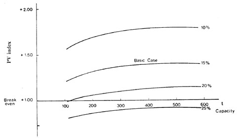
Figure 7.8 Influence of Change in Rate of Discount. Pelagic Fishing Boats in Peru, according to Engstrom et. al (1974)
At a rate of 20%, boats with less than 200 t capacity are not profitable, while no boat can realize profits if the rate rises to 25% (Engstrom et al., 1974).
The following are different economic analyses for various small and medium sized fish plants. An economic analysis was made of small fish canning plants in tropical countries, for the production of 10 000 (model 1) and 20 000 (model 2) cans of 125 g of sardines every 8 hours. The substitution of machinery (model 1) for labour (model 3) was also evaluated at the same time.
Table 7. 11 shows the values resulting from the application of the internal rate of return and present-worth methods, utilizing a discount rate of 10 % for the last method, which is the rate adopted by the Tropical Products Institute in project evaluation. A useful life of 10 years was considered.
Table 7.11 Evaluation of Profitability for Small Fish Canning Plants
Present-worth (i = 10%) (US$) Internal rate of return (r) |
Model 1 1262100 61.5% |
Model 2 2678910 69.5% |
Model 3 1153382 59.0% |
A) 200 days/year 150 days/year |
47.5% 33.5% |
54.0% 38.5% |
45.0% 31.5% |
B) 50% to domestic market |
33.5% |
39.0% |
29.5% |
C) +25% Production costs |
36.7% |
42.6% |
32.0% |
A sensitivity analysis was also made using the following parameters: (A) reduction of working days per year (200 and 150); (B) 50% of the production is sold in the domestic market; (C) 25 % increase in operating costs. The base model considered 250 days/year and 100% of production designated for export, where prices higher than those of the domestic market (60%) could be obtained.
The internal rate of return (r) decreases by an average 38.5%. If the first two parameters are considered together, the values found are lower by 50% and results are negative when the third factor is incorporated (Edwards et al., 1981). Table 7.12 shows the investments required and the IRR for fish and shellfish canning plants in Indonesia (Bromiley et al., 1973).
Table 7.12 Internal Rate of Return (r) for Fish Canning Plants in Indonesia
Location |
Annual Capacity (in '000 cans) |
Total Investment (US$) |
r (%) |
Bitung |
104 (tuna) |
1 850 000 |
36 (*) |
Pare-Pare |
720 (tuna) |
360 000 |
35 |
Central Java |
3 840 (shrimp) |
810 000 |
45 |
(*) Calculation of the internal rate of return (r) is affected by the interest that must be paid by the investment; if half of the investment is financed by a 10 year loan with an 12% interest rate, the value of the internal rate of return would be 52%.
The internal rate of return calculated for mechanized canning plants in Norway, with a production capacity of 15 t/day of raw material (sardines), was 27. 1 % (Myrseth, 1985). There are evaluations where it is practical to express the results as a function of variables whose estimates are uncertain. For example, the economic performance of freezing plants for whole fish block was studied in order to calculate the price that should be paid for raw material, if favourable internal rates of return of 10 and 20% were considered, along with a useful life of 15 years for the investments. Table 7.13 summarizes the results.
Table 7.13 Price of Raw Material Calculated for Internal Rates of Return of 10 and 20%
Raw Material Price (US$/t) |
||
r = 10% |
r = 20% |
|
Annual
Production: 2 240 t |
|
|
Annual
Production: 3 360 t |
|
|
Two production levels were studied. In the first case, 2 240 t of whole fish were used annually, with two 8-hour shifts per day, working 250 days; in the second, 3 360 t were used, with an additional 8-hour shift and increased refrigeration and ice plant capacity. If the energy costs decrease by 50%, the purchase price of the raw material could rise by US$ 17/t. An internal rate of return for a hypothetical case involving a fishmeal plant, with an investment of US$ 10 000 (over a 5-year period) was calculated at 18.5 % (FAO, 1986a). In small fish smoking plants, the distribution of profits is similar to that used by artisanal fishermen. The income received from the operations of the plant is shared equally among the workers in the plant, with one share for the "association", once operational costs have been deducted. As the plant functions with three workers, the income is divided into four parts; one for each worker and one for the Trade Union Association (FAO, 1986a).
In Sri Lanka, an evaluation was made of the production of liquid silage for a plant with an annual capacity of 450 t of product, at three different sales prices, taking a value of US$ 333/t and depreciation percentages of 20 and 25 %. Determination of the internal rates of return for a useful life of 5 years resulted in values of 77, 38 and 26% respectively. These figures indicate that the project would be highly profitable (Aagaard et al., 1980) (Disney & James, 1980).
Another economic analysis shows the production of liquid silage from shrimp by-catch in Mexico. The fixed investment rises to US$ 28 289 and the working capital to US$ 6 667 for an annual production of 312 t of silage. The production costs are US$ 92/t taking into account an amortization period of five years. The sales price was calculated using an internal rate of return of 15 %. The price for silage showed significant advantages when compared to the prices of other sources of proteins and fishmeal. It should be added that the cost per unit of protein is profitable, even when species and inputs (acid) at higher prices are used in the production (Edwards and Disney, 1980). In general, it would appear that the production of liquid silage is profitable, but special consideration must be taken of the distance of the factory from the consumers and the competitive prices of other feeds. There is no question of the nutritional advantage of its use in the formulation of feed for pigs (Bertullo, 1989; Andrade et al., 1992; Bello et al., 1992), and the possibility of its utilization in animal feeds for birds, fur animals, cultured fish and calves.
It is useful to study the influence of profitability on each component of income, expenditure and investment, as a complement to profitability studies. This information will enable fundamental adjustments to be made to those parameters that show greatest influence, leaving the other parameters to a less ambitious estimate.
In a sensitivity analysis several variables with reasonable designs are selected, and are varied at successive stages, through an allowable percentage of variation. The resulting variations in the profitability indicate the importance of each variable investigated.
Example 7.10 Sensitivity Analysis
Make a sensitivity analysis for a canning plant, using the conditions for the basic case given in Table 7.14. The relative parameter is defined as the relationship between the real value of the parameter and its value in the example, calculating the relative change of the Internal Rate of Return in the same manner.
Table 7.14 Assumptions for the Basic Case
1 |
Production speed is equal to annual sales |
2 |
Plant capacity: 100 000 (cans/day) |
3 |
Working capital as empirical function of fixed investment, operating costs and sales |
4 |
Depreciation by straight-line method |
5 |
Estimated useful life: 10 years |
6 |
Taxation rate: 45% (average value for Argentina) |
7 |
Zero residual value |
8 |
No financial costs |
9 |
150 days/production year (average for canning plants in Argentina) |
10 |
Selling price remains constant while other parameters vary |
Answer:
Table 7. 15 and Figure 7.9 show the results of the sensitivity analysis.
Small variations in the sales price and costs of raw material (fish and packaging) modify the profitability of the plant to a considerable extent. This would indicate that for a quick estimate of costs and profitability, these data be known exactly, even when precise data are not available on plant capacity, labour, utilities and fixed costs. Raw material requirements must be calculated as precisely as possible and an accurate market study undertaken to determine the sales price. This is particularly true for processes that are not capital-intensive, that is, those processes that are controlled by variable costs. Here, the effect of sale price on profitability is approximately double that of the other parameters (Cerbini and Zugarramurdi, 1981a).
Table 7.15 Sensitivity Analysis
Number in Figure 7.5 |
Parameter |
Variation in Parameter |
Relative Value of Internal Rate of Return |
1 |
Selling Price |
+10 - 4 |
1.90 0.57 |
2 |
Rate of Production |
+20 -20 |
1.14 0.88 |
3 |
Raw Material Price |
+15 - 15 |
0.58 1.35 |
4 |
Price of Can |
+15 - 15 |
0.28 1.56 |
5 |
Investment |
+ 20 -20 |
0.64 1.20 |
6 |
Days per year |
+ 47 -25 |
1.29 0.83 |
7 |
Costs of Labour |
+20 -20 |
0.63 1.31 |
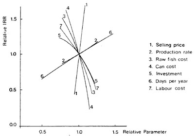
Figure 7.9 Sensitivity Analysis for Canned Anchovy, Argentina 1981
Inflation is an economic phenomenon feared worldwide; developed countries monitor it closely and the anticipated and actual inflation are in the news at least once a month. In many developing countries inflation effects are often endured. Inflation can be due to a number of reasons, usually linked to macro-economics decisions and politics, such as emission of currency without the proper support. Additional information on the concept of inflation is given in Appendix B.5. Table 7.16 shows series of inflation rates in several Latin American countries where a permanent occurrence of high values (2 and 3 digits) are observed. Inflation indicators are based on particular mixtures of goods and services chosen to represent the material needs of an average citizen.
Table 7.16 Consumer Price Index (average increase % per year)
Year |
Argentina |
Bolivia |
Brazil |
Colombia |
Chile |
Mexico |
Uruguay |
1976 |
444.1 |
4.5 |
35.7 |
17.4 |
211.8 |
15.8 |
50.6 |
1977 |
176.0 |
8.1 |
40.5 |
28.6 |
91.9 |
28.9 |
58.1 |
1978 |
175.5 |
10.4 |
38.3 |
18.7 |
40.1 |
17.5 |
44.5 |
1979 |
159.5 |
19.7 |
50.2 |
24.2 |
33.4 |
18.2 |
66.8 |
1980 |
100.8 |
47.2 |
77.9 |
27.9 |
35.1 |
26.3 |
63.5 |
1981 |
104.5 |
32.2 |
95.6 |
29.4 |
19.7 |
28.0 |
34.1 |
1982 |
164.8 |
92.0 |
89.6 |
23.4 |
9.9 |
58.9 |
19.9 |
Source: (Index Econ6mico, 1984); (Coyuntura y Desarrollo, 1983)
Given the wide calculating basis, these indexes represent a reasonable estimate of the inflation rate for other economic activities. Such inflation is termed "general" where, it is assumed, all economic sectors increase their prices at the same rate, contrary to so-called "repressed" or "differential" inflation, where, for several causes such as technological changes, shortages of a few raw materials, government policies, etc., the different factors of the economy may inflate at unequal rates. In countries with extreme inflation rates, the "differential" deviations become less important and may be ignored. This can be observed in Table 7.17 which presents a series of inflation indexes for Argentina.
Table 7.17 Price Evolution Indicators in Argentina (1970 base = 1)
Consumer Price |
Index |
General Index |
Construction Cost Index |
Wholesale Price Index |
Agricultural Price Index |
||
Materials |
Labour |
General Expenses |
|||||
1970 |
1.00 |
1.00 |
1.00 |
1.00 |
1.00 |
1.00 |
1.00 |
1971 |
1.391 |
1.432 |
1.419 |
1.457 |
1.357 |
1.482 |
1.602 |
1972 |
2.284 |
2.268 |
2.393 |
2.158 |
2.253 |
2.608 |
3.002 |
1973 |
3.283 |
3.659 |
3.623 |
3.742 |
3.426 |
3.41 |
3.506 |
1974 |
4.598 |
5.98 |
6.343 |
5.816 |
5.283 |
4.642 |
4.259 |
1975 |
20.006 |
28.604 |
36.923 |
21.514 |
26.892 |
20.807 |
16.923 |
1976 |
89.536 |
91.00 |
136.27 |
50.836 |
88.822 |
101.18 |
94.593 |
1977 |
233.18 |
204.63 |
330.48 |
96.67 |
191.032 |
250.07 |
218.08 |
1978 |
629.22 |
517.14 |
810.69 |
262.81 |
475.89 |
608.43 |
557.60 |
1979 |
1 508.46 |
1 251.50 |
2036.11 |
567.61 |
1 159.61 |
1 392.45 |
1 203.12 |
1980 |
2 830.40 |
2527.30 |
3 905.96 |
1 300.63 |
2481.07 |
2 192.57 |
1 637.98 |
1981 |
6545.96 |
5 247.30 |
8 320.66 |
2611.65 |
4768.25 |
6 143.51 |
5 123.00 |
1982 |
20276.10 |
19322.70 |
31 635.40 |
9 167.80 |
15 881.40 |
25268.50 |
21 209.50 |
1983 |
108208.90 |
127361.00 |
181936.00 |
79248.90 |
104 299.00 |
129013.00 |
103 829.60 |
ß |
93.50 |
93.50 |
100.90 |
83.30 |
91.60 |
94.30 |
91.801 |
ß Average Inflation Index (by least-squares)
Even in this period of intense social and economic change, indicated in Table 7.17 the differences between various sectors did not exceed 10% as can be observed in the last row ß of Table 7.17.
Although it seems that most countries, including developing countries, are now (1995) moving towards a more stable (and less inflationary condition), fish processing companies operate in the real world, and therefore they may have to strive to survive under inflation conditions. Inflation affects calculations of profitability of investment projects, causing the analysis and the decision-making to become difficult and confused. This is especially true in countries where high inflation rates are virtually constant, as was the case of Argentina and other Latin American countries.
This section will deal exclusively with the influence of general inflation on the profitability analysis of a project, showing the difference between real profit and that which can only be qualified as a numerical result product of an inflationary process.
The use of stable currency for cash flow values is a usual procedure to find values of "real internal rate of return". However, in considering components of cash flow which are independent of the inflation rate, such as amortization of loans and the real value of working capital, the application of cash flow values in stable currency for the calculation of a real IRR is not valid and the formulas described must be modified (de Santiago et al., 1987).
The effect of the consideration of inflation on the Present-Worth and Internal Rate of Return Methods are first analysed by applying them to the example of the freezing plant.
Equation (7. 11) is valid for the case of zero inflation. In the case where inflation has a fractionary rate this equation can be written as:
(7.25)
When ß = 0, the equation (7.25) is the same as (7. 11) with iR (real rate) = i
Example 7.11 Calculate the Present-Worth (PW) (taking inflation into consideration)
Calculate the Present-Worth (PW) for the hake freezing plant in Example 7. 1. Use an annual inflation rate of 80%, assuming that the plant is located in Argentina.
Answer: The exchange rate is 10 000 Australes/US$ 1 (1990). Therefore, if Table 7.1 is expressed in Australes, the values will be those shown in Table 7.18.
Applying Equation (7. 11), the present-worth of the project at the end of year 10 is 1 102 million Australes.
PW = (7.702 - 6.60) x 109 = 1.102 x 10⁹, so: PW = 1 102 million Australes
Table 7.18 Statement of Sources and Application of Funds for a Fish Plant when there is no Inflation (in '000 million Australes (A)
Activity |
90 |
91 |
92 |
93 |
94 |
95 |
96 |
97 |
98 |
99 |
SOURCE |
|
|
|
|
|
|
|
|
|
|
Own capital |
4.8 |
|
|
|
|
|
|
|
|
|
Bank credit (*) |
1.8 |
|
|
|
|
|
|
|
|
|
Net Sales from activity |
8.42 |
8.42 |
8.42 |
8.42 |
8.42 |
8.42 |
8.42 |
8.42 |
8.42 |
8.42 |
Total (a) |
15.02 |
8.42 |
8.42 |
8.42 |
8.42 |
8.42 |
8.42 |
8.42 |
8.42 |
8.42 |
APPLICATIONS |
|
|
|
|
|
|
|
|
|
|
Fixed Investment |
6.0 |
|
|
|
|
|
|
|
|
|
Working Capital |
0.6 |
|
|
|
|
|
|
|
|
|
Cost of Financing (**) |
0.27 |
|
|
|
|
|
|
|
|
|
Cost of Production |
6.87 |
6.87 |
6.87 |
6.87 |
6.87 |
6.87 |
6.87 |
6.87 |
6.87 |
6.87 |
Total (b) |
13.74 |
6.87 |
6.87 |
6.87 |
6.87 |
6.81 |
6.97 |
6.87 |
6.87 |
6.87 |
(a) - (b) |
1.29 |
1.56 |
1.56 |
1.56 |
1.56 |
1.56 |
1.56 |
1.56 |
1.56 |
1.56 |
Net Profit (***) |
0.77 |
0.93 |
0.93 |
0.93 |
0.93 |
0.93 |
0.93 |
0.93 |
0.93 |
0.93 |
Plus depreciation |
0.60 |
0.60 |
0.60 |
0.60 |
0.60 |
0.60 |
0.60 |
0.60 |
0.60 |
0. 60 |
Cash Flow |
1.37 |
1.53 |
1.53 |
1.53 |
1.53 |
1.53 |
1.53 |
1.53 |
1.53 |
1.53 |
(*) 30% IF = A 1 800 million (**) 15% Annual Rate (***) Deducting taxes on earnings (40%)
The example could be modified using an 80% annual inflation rate, but disregarding the effect of inflation and incorrectly applying Equation 7. 11. The data for this situation are given in Table 7.19, and results in a present-worth of 221 800 million Australes.
Table 7.19 Statement of Sources and Applications of Funds for a Fish Plant with Inflation (ß = 0.8) (in '000 million Australes (A)
Activity |
90 |
91 |
92 |
93 |
94 |
95 |
96 |
97 |
98 |
99 |
SOURCE |
||||||||||
Own capital |
4.8 |
|||||||||
Bank credit (*) |
1.8 |
|||||||||
Net Sales from activity |
15.2 |
27.3 |
49.1 |
88.4 |
159.2 |
286.5 |
515.7 |
928.3 |
1671.0 |
3007.8 |
Total (a) |
21.8 |
27.3 |
49.1 |
88.4 |
159.2 |
286.5 |
515.7 |
928.3 |
1671.0 |
3007.8 |
APPLICATIONS |
||||||||||
Fixed Investment |
6.0 |
|||||||||
Working Capital |
0.6 |
|||||||||
Cost of Financing (**) |
0.5 |
|||||||||
Cost of Production |
12.4 |
22.3 |
40.1 |
72.1 |
129.8 |
233.6 |
420.5 |
756.9 |
1362.5 |
2452.5 |
Total (b) |
19.4 |
22.3 |
40.1 |
72.1 |
129.8 |
233.6 |
420.5 |
756.9 |
1362.5 |
2452.5 |
(a) - (b) |
2.3 |
5.0 |
9.1 |
16.3 |
29.4 |
52.9 |
95.2 |
171.4 |
308.5 |
555.3 |
Net Profit (***) |
1.4 |
3.0 |
5.4 |
9.8 |
17.6 |
31.7 |
57.1 |
102.8 |
185.1 |
333.2 |
Plus amortization |
0.6 |
0.6 |
0.6 |
0.6 |
0.6 |
0.6 |
0.6 |
0.6 |
0.6 |
0.6 |
Cash Flow |
2.0 |
3.6 |
6.0 |
10.4 |
18.2 |
32.3 |
57.7 |
103.4 |
185.7 |
333.8 |
(*) 30% IF = A 1 800 million (**) 15% Annual Rate (***) Deducting taxes on earnings (40%)
PW = (281.2 - 6.60) x 109 = 274.6 x 10⁹, so: PW = 274 600 million Australes
Taking inflation into account and correctly applying Equation (7.25) yields a totally different result, and reveals that the project actually has a negative PW.
PW = (5.251 - 6.60) x 109 = -1.349 x 10⁹, so: PW = -1 349 million Australes
This example shows that the effect of inflation is to make a project appears more profitable than it really is.
This could be the case of many past investment failures in developing countries.
Inflation affects the calculation of profitability of investment projects, making analysis and decision-making difficult, especially in those countries where high levels of inflation predominate. In turn, it negatively affects investment possibilities.
The well-known concept of real rate of interest (Riggs, 1977; Barish and Kaplan, 1978) will be used which, is based on the following reasoning: Consider a trust Io which for a year has yielded an interest (Io x i); then the total amount I1 will be:
I1 = Io x (1 + i) (7.26)
If in this period there was an inflation rate b , the relationship between the real value of I1, (designated I10) and the value of Io would be:
I10 = I1 / (1 +ß) = Io x (1 + i) /(1 + ß) (7.27)
A real rate of interest iR (taking into account the effect of inflation) (Jelen and Black, 1983; Jones, 1982) could be defined by the expression:
I10 = Io x (1 + iR ) (7.28)
Equating the expressions Equation (7.27) and (7.28), the following can be deduced:
(7.29)
This formula differs from that commonly used:
iR ~(real approximate rate of return) = i - ß (7.30)
which is only valid when b < < 1, (Holland
and Watson, 1977; Estes et al., 1980; Shashua and Goldschmidt,
1985). It gives an estimate of the real rate of interest higher
than those defined by Equation (7.29). Having defined the
relative error (![]() )
by Equation (7.31), it was found to coincide with the inflation
rate:
)
by Equation (7.31), it was found to coincide with the inflation
rate:
(7.31)
Introducing the concept of real rate of interest, defined by Equation (7.29), a real internal rate of return is determined when Equation (7.32), referring to discounted cash flow, is equal to zero:
(7.32)
where CFj is the net cash flow in year j and n is the number of periods in the project life. If the economy is affected by a phenomenon of general inflation the numerator of each term of the sum is assumed to have been expanded by the inflation rate:
(7.33)
When adding Equation (7.33) to (7.32), it can be observed that the utilization of cash flow in constant value terms leads to the values of "real internal rate of return" (IRR).
Example 7.12 Calculation of Internal Rate of Return, IRR (r)
Calculate the internal rate of return for the hake freezing plant of Example 7. 1. Use an 80% rate of annual inflation.
Answer:
From Table 7.19, a value of r = 96.9% is obtained. Calculating the IRR from the Net Cash Flow corrected by inflation, an iR Of 11 % is obtained. From Equation (7.29):
This result shows once again the effect of inflation on a case that appeared profitable, when inflation is not taken into account. However, in practice, several components of cash flow can be independent of the inflation rate, such as: amortization of loans, payments of interest, payment of taxes, adjustments to working capital, etc.; thus preventing the use of cash flow in constant currency for the calculation of a real IRR.
To face the inflation problem, some of these concepts will be analysed in a simple cash flow consisting of an initial investment yielding a constant cash flow when the inflation rate is zero during a planning horizon of 10 years.
The inflation obliges to increase the working capital Iw. To study the effect of this increment on the profitability, it is assumed that the working capital may be expressed in fractions (f Iw) on the annual sales "S". Taking into account that the annual sales (S) and the annual operating costs (C) are expanded by the inflation:
(7.34)
but there could be the need of an annual increase of working capital by:
(7.35)
and the capital accumulated would be recovered at the end of the year N
(7.36)
As a result, the IRR formula (before taxes) is transformed into:
(7.37)
and with little change:
(7.38)
and the following equation is derived:
(7.39)
The effect of the inflation on the real profitability iR by the devaluation of the working capital is expressed by Equation (7.38). To analyse such influence the following dimensionless relationships are substituted in Equation (7.38):
R = So /Co and X = Co / Io
and the whole equation is divided by Io, thus giving the final expression:
(7.40)
A panorama of the inflation showing the different parameters that includes Equation
(7.40) is illustrated in Table 7.20.
Table 7.20 Real Internal ate of Return
Gp* |
IW |
b =0 |
0.2 |
0.5 |
1.0 |
1.5 |
2.0 |
4.0 |
0.3 |
0.1 |
0.2447 |
0.2269 |
0.2089 |
0.1906 |
0.1794 |
0.1719 |
0.1567 |
0.5 |
0.1 |
0.4440 |
0.4280 |
0.4120 |
0.3958 |
0.3861 |
0.3795 |
0.3665 |
0.7 |
0.1 |
0.6320 |
0.6166 |
0.6011 |
0.5855 |
0.5762 |
0.5700 |
0.5575 |
Note:
Table 7.20 shows that the real rate of return is deteriorated by inflation. This reduction becomes more pronounced as the working capital acquires more relative importance. In order to maintain the profitability of a company, the immediate action of managers should be to increase the selling price of the products in relation to the costs, assuming that this could be possible without reducing the sales volume.
This strategy is represented by Equation (7.41) by R' R. In order to maintain the constant 'R resulting in Equation (7.41), the proportional increase (R'/R) can be obtained by Equation (7.40) with ß = 0 and the value of the original R.
(7.41)
For a "before-tax profitability" iR = 0.3, values from Equation (7.41) are shown in Figure 7. 10. It can be observed from Figure 7. 10 that the appropriate factor can reach high values, and when there is an increase in prices producing a multiplying effect over inflation indexes.
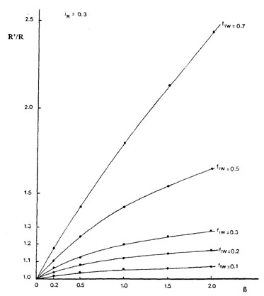
Figure 7. 10 Selling Price Increasing Ratio (R'/R) vs Inflation Rate (ß) at Different Percentages of Working Capital, a Constant Profitability iR=0.3 is Considered
An analysis using a continuous formula is appropriate in the case of the working capital devaluations, due to high rates of inflation, so the adjustments must be made in shorter time periods. For continuous interest, simple deductions yield the following relationships:
Future value: F(t) = F(o) x exp(i x t) (7.42)
Future value in constant currency: Fo(t) = F(o) x exp(i x t) x exp(- b x t) (7.43)
Definition of real rate of interest: Fo(t) = F(o) x exp(iR X t) (7.44)
It is important to note that in the continuous case the approximate Equation (7.30) is valid. The resulting equation for calculating the IRR without inflation is given by:
(7.45)
where the i that makes zero the equality in Equation (7.45) is the internal rate of return (IRR). When inflation is taken into account, the following definitions will be used:
(7.46)
(7.47)
(7.48)
(7.49)
With those expressions, the equation that defines the real internal rate of return will be:
(7.50)
Introducing the concept of real rate of interest (continuous case iR = i - b ), the integrated equation is:
(7.51)
Using the relationships X and R, and dividing by Io, the Equation (7.51) is transformed into (7.52), that is the continuous expression equivalent to Equation (7.40).
(7.52)
and the continuous expression of (R'/R) corresponding to (7.4l):
(7.53)
The "continuous" Equations (7.52) and (7.53) show an unfavourable effect compared with their similar annual discrete forms and this is more noticeable as the inflation rate increases. Continuous equations show that in a profitability analysis the study with annual period can lead to serious mistakes. For certain inflation rates, analysis of Equation (7.53) shows that for high fIw values of R'/R allowing a reasonable profitability would not be possible. In consequence, the enterprises must decrease their working capital and accept lower profitability. The persistence of the inflation phenomenon would lead to capital losses.
Some sectors of the economy have no possibility of modifying the selling price of their products, such as in the case of exporting industries or in open economies with perfect competition from foreign countries. In such instances, another available resource is the utilization of loans which can improve or deteriorate the project profitability according to the stipulated rate of interest. Furthermore, the amount of the investment made by the firm is reduced, changing also the IRR.
There is a large variety of loan types, therefore only those which permit some generalizations will be analysed. First, the financing of the working capital year by year will be analysed; that is, a loan must be totally amortized in a period j
fIw × So × (1 + ß )j-1
paying a rate of interest i~ and taking out a new loan:
fIw ×So × (1 + ß )j
In this case the equation that defines the IRR is as follows:
(7.54)
or with the dimensionless relationship:
(7.55)
Equation (7.55) is obtained from Equation (7.40) using b = 0, and it shows the maximum rate of interest i~ that would be paid for financing the working capital while keeping a constant profitability equal to the zero inflation case.
iP = iR × (1 + ß ) (7.56)
For some cases studied in Table 7.20, figures of ip calculated from Equation (7.56) are presented in Table 7.21. If a constant profitability is desired, an interest rate higher than inflation could only be paid at low inflation rates. At higher inflation rates, lower interest rates (including negatives) must be paid. Even though it is useless to maintain the level of profitability, the financing of the working capital by loans at an interest rate lower than total project profitability (including inflation), would yield a net improvement on the real profitability, but the loss from inflation does not suffice when the values given from Equation (7.56) do not reach that project profitability.
Table 7.21 Rates of interest (ip) for Financing Working Capital at Constant Profitability
GP* |
IW* |
iR=0 |
b =0.2 |
0.5 |
1.0 |
1.5 |
2.0 |
0.3 |
0.7 0.5 0.3 0.1 |
0.1471 0.1703 0.2013 0.2447 |
0.1765 0.2043 0.2418 0.2436 |
0.2206 0.2554 0.3019 0.3670 |
0.2942 0.3406 0.4026 0.4894 |
0.3677 0.4257 0.5032 0.6117 |
0.4413 0.5109 0.6039 0.7341 |
0.5 |
0.7 0.5 0.3 0.1 |
0.2788 0.3191 0.3720 0.4440 |
0.3345 0.3829 0.4464 0.5328 |
0.4182 0.4786 0.5580 0.6660 |
0.5576 0.6382 0.7440 0.8880 |
0.6970 0.7977 0.9300 1.1100 |
0.8364 0.9573 1.116 1.3320 |
From the cases presented in Table 7.20, real profitability that could be reached by financing the working capital at rate of interest iP = ß (neutral real rates of interest) are shown in Table 7.22, observing important improvements with respect to those values given in Table 7.20.
Table 7.22 Rate of Profitability with Financing of Working Capital with Neutral Rates
GP* |
IW* |
b =0.2 |
0.5 |
1.0 |
1.5 |
2.0 |
4.0 |
0.3 |
0.1 |
0.2538 |
0.2341 |
0.2141 |
0.2018 |
0.1936 |
0.1768 |
|
0.3 |
0.2141 |
0.1510 |
0.0814 |
0.0346 |
- |
- |
|
0.5 |
0.1726 |
0.0560 |
- |
- |
- |
- |
|
0.7 |
0.1287 |
- |
- |
- |
- |
- |
0.5 |
0.1 |
0.4733 |
0.4558 |
0.4381 |
0.4275 |
0.4204 |
0.4061 |
|
0.3 |
0.4381 |
0.3845 |
0.3298 |
0.2961 |
0.2732 |
0.2262 |
|
0.5 |
0.4025 |
0.3111 |
0.2141 |
0.1510 |
0.1056 |
0.0000 |
|
0.7 |
0.3664 |
0.2341 |
0.0814* |
- |
- |
- |
0.7 |
0.1 |
0.6795 |
0.6625 |
0.6455 |
0.6353 |
0.6285 |
0.6148 |
|
0.3 |
0.6455 |
0.5943 |
0.5428 |
0.5117 |
0.4908 |
0.4487 |
|
0.5 |
0.6114 |
0.5255 |
0.4381 |
0.3845 |
0.3482 |
0.2732 |
|
0.7 |
0.5772 |
0.4557 |
0.3298 |
0.2499 |
0.1936 |
0.0064 |
The utilization of a loan financing a percentage of total investment amortized in equal shares at constant currency (a loan with indexed payments) will be analysed. It is assumed that amortization of the loan will be in N payments, where:
N = economic life of the project
Amount of the loan p x Io ; 0 < p < 1
Amortization: Aj = p x Io x Fp (ip,N) x (1 + ß)j
i.e., the annuity factor. It follows that the real internal rate of return is the root of the following dimensionless equation:
(7.57)
The stipulated interest is equivalent to the real internal rate of return of an equivalent investment to the amount borrowed. Then, it is obvious that if the ip < iR, where iR is the project profitability without the loan from a borrower's viewpoint, the profitability would improve. Nevertheless, as the inflation increases and the profitability decreases below the interest rate of the loan, the latter can be made highly onerous. A contrary effect is observed for iR < 0. 1 in the result presented in Table 7.23, where iR is the project profitability with a loan at an interest rate ip = 0. 1.
Table 7.23 Variation of the Real Rate of Return vs Inflation Rate for Indexed Loans on Investment
p = 0.7 |
b = 0 |
0.2 |
0.5 |
1.0 |
1.5 |
2.0 |
4.0 |
Case 1 |
|||||||
GP* = 0.3 |
iR = 0.2013 |
0.1554 |
0.1072 |
0.0559 |
0.0230 |
- |
- |
IW* = 0.3 |
iR' = 0.2983 |
0.2083 |
0.1142 |
0.0130 |
-0.0530 |
- |
- |
Case 2 |
|||||||
GP* 0.5 |
iR = 0.3191 |
0.2586 |
0.1960 |
0.1306 |
0.0893 |
0.0607 |
0.00002 |
IW* = 0.5 |
iR' = 0.4789 |
0.3723 |
0.2637 |
0.1518 |
0.0820 |
0.0338 |
-0.06780 |
Case 3 |
|
||||||
GP* = 0.7 |
iR = 0.4035 |
0.3313 |
0.2575 |
0.1810 |
0.1333 |
0.1004 |
0.0314 |
IW* = 0.7 |
iR' = 0.5843 |
0.4663 |
0.3472 |
0.2259 |
0.1514 |
0.1006 |
-0.0045 |
Rate of interest of the loan i, 0. 1
To improve profitability, the interest rate of a loan must be less than the total internal rate of return (including the real rate plus the inflation rate), irrespective of whatever amortization scheme is applied. This conclusion can be deduced from a study on the following dimensionless equation:
(7.58)
where it has been considered:
Amount of loan p x Io 0 < p < 1
Amortization: Aj = p x Io x Fp (ip,N)
The fact that iR' iR when it is i ip is shown in Table 7.24. This type of loan would have little difficulty to face possible increases in the inflation rate.
Table 7.24 Variation of the Internal Rate of Return vs Inflation Rate for Non-Indexed Loans Rate of Interest of the Loan ip= 0.72; Financed Investment Fraction p = 0.70
b = 0 |
0.2 |
0.5 |
1.0 |
1.5 |
2.0 |
4.0 |
|
Case 1 |
iR = 0.2013 |
0.1554 |
0.1072 |
0.0559 |
0.0230 |
- |
|
GP* = 0.3 |
i = 0.2013 |
0.3865 |
0.6608 |
1.1118 |
1.5575 |
- |
- |
IW* = 0.3 |
iR' = - |
0.01009 |
0.0938 |
0.1037 |
0.0908 |
- |
- |
Case 2 |
iR = 0.3191 |
0.2586 |
0.1960 |
0.1306 |
0.0893 |
0.0607 |
0.00002 |
GP* 0.5 |
i = 0.3191 |
0.5103 |
0.7940 |
1.2612 |
1.7232 |
2.1821 |
4.0001 |
IW* = 0.5 |
iR' = 0.4789 |
0.1774 |
0.2115 |
0.1914 |
0.1632 |
0.1388 |
0.07755 |
Case 3 |
iR = 0.4035 |
0.3313 |
0.2575 |
0.1810 |
0.1333 |
0.1004 |
0.0314 |
GP* = 0.7 |
i = 0.4035 |
0.5976 |
0.8862 |
1.3620 |
1.8332 |
2.3012 |
4.157 |
IW* = 0.7 |
iR' = 0.5843 |
0.4663 |
0.2893 |
0.2468 |
0.2075 |
0.1764 |
0.1030 |
In the case of high rates of inflation, the phenomenon of general inflation of all factors which are involved in the discounted cash flow predominates, and the use of values in stable currency leads to a determination of the real internal rate of return. However, inflation produces a need for continuous contributions to working capital which causes reductions in the profitability that can reach relatively high values.
This can be corrected, where possible, through increases in the margin of sales, or by use of loans. In this case it has been shown that its effectiveness is lost as inflation increases, and can lead to adverse effects. In particular, indexed loans (among which, foreign currency loans whose rate of exchange follows the rates of general inflation) pose a high risk, since, if the inflation rate were increased, considerable losses would occur.
The equations obtained for cash flows with results repeated over time quantify these concepts, presenting values calculated in tables as a function of dimensionless parameters which represent the relationship of sales over operating costs, operating costs over fixed investment and working capital over sales. A generalization of the continuous case would indicate the need for short-term analyses, since analysis in annual periods could lead to wide errors in the case of high rates of inflation.
The generalized commercial practice of increasing the sales margin (to cover the replacement cost), would lead to a self sustained inflationary process, which is difficult, if not impossible, to control through the mechanisms of classic economics.
The combination of all these factors, with annual variable output and variable rates of inflation, can only be resolved through a discounted cash flow, including the concept of real profitability defined by expression (7.32). However, the formulas presented as a function of dimensionless parameters give a useful general idea of decision-making on strategies to be used in the event of high inflation rates.
High inflation rates, or just inflation, it is not a situation usually sought or desired by an industry, but a situation to be faced and overcome in order to survive. From experience in countries with high inflation rates, it is clear that most of the management effort in such situations is directed towards developing financial strategies in order to survive. Other aspects, like market and technological development and quality, receive less or no attention. Unfortunately, relatively high inflation rates continue to be a problem in many developing countries. Therefore it has been found necessary to include this analysis - certainly not restricted to the fishery industry - to provide appropriate tools to the interested reader.
![]()
![]()
![]()