2.1 Plant Capacity and Location
2.1.1 Information required from market studies
2.1.2 Plant location
2.2
Required Technical Information
2.3
Production Technologies for Fishery Products
2.4 Input Requirements
2.4.1 Raw material
2.4.2 Ice consumption
2.4.3 Labour
2.4.4 Utilities
2.4.5 Packaging
Production engineering is a vital element when conducting an economic evaluation of a process. It is applied in the project phase of an industry and is an analytical tool when production has started and deviations from the initial project appear or when modifications to the installed processes are required. When the final design phase of a process in a new project is completed, or when all technical data concerning a process in an existing plant have been collected, it is then possible to estimate the costs, as detailed specifications of equipment and complete information on the needs of the plant will be available.
First, those aspects relating to plant capacity for each of the products to be made must be analysed. For a project, examination of factors such as engineering, investments and locations, will assist in reducing the number of alternatives for selection.
The size and characteristics of the target market provide the first indication to define production level and hence investment. This manual does not analyse markets in general and fish markets in particular. It does not underestimate the market component; and the importance of having appropriate market information to start or expand any industrial endeavour is recognized.
Market information is necessary to define production level, type of products, required technology, type of packaging, etc. In practice any industrial development starts with a number of questions: How many tons of a product can be sold? At what price? To whom? What is the current supply? The answers to these questions can be found by conducting a market survey which will establish the size of the market by estimating the quantity of a particular product that will be in demand, and its price (Samuelson, 1983). A more complete analysis of market trends can be done by studying variations in demand in relation to income, prices, demographic factors, changes in the geographic distribution of the market, and the influence of the market size on costs. As examples of this type of approach, two cases (Hotta, 1979; and Raizin and Regier, 1986) are discussed in Appendix A.
In the fishery industry, an initial analysis of the size of the market is, usually made according to the first, simpler method, as it is often difficult to access data at national or international level to produce a more exhaustive study. It must be underlined that the more information obtained on the prospective market, the better. The concept that supply adapts to demand is universally accepted. What is less apparent is that an exact understanding of the supply-demand relationship is the first step in understanding the operation of the whole economic system. A high demand or supply of a product can be created by factors other than those of the market. Governments, for political or social reasons, can decide that certain prices are too high or low and take action to establish maximum or minimum prices or impose taxes. Without analysing the advantages or disadvantages of these restrictions, the supply-demand relationship will reveal why they create scarcity or abundance.
Three markets are involved in a distribution system: markets for inputs, for fresh fish, including intermediate products (such as frozen fish), and for the final product. In the first market, variable inputs (ice, bait, labour) and fixed inputs (engines, fishing gear) are bought by fishermen, who convert them into fishing effort, which results in a quantity of landed fish. The fisherman's demand for inputs such as ice and bait, is derived from the anticipated sale of fish. In the second market, the processors buy, process and transport the fresh fish, and incur costs in the use of ice, transport, buildings and freezers. Demand for fresh fish by the processors in small-scale fisheries is derived from their anticipated income from a third market; that is, sale of their processed product to the consumers.
The dynamism of fish markets makes them difficult to define. This dynamism is due mainly to the seasonality of the catch within a year, and the changes in volume and composition of catch from one year to another. In the medium and long terms, the market for fish is also influenced by changes in eating habits, the introduction of new species, economic reasons such as the increasing cost of labour, or technological factors such as the lack of adequate packaging or the difficulty in running an efficient distribution system.
The quantity of fish distributed by the fishing sector to consumers over a period of time depends on many factors. Basically it depends on the type of resource and method of extraction, quantity of fish caught, quantity of fish demanded by the consumer, existence of flaws in the three markets, in infrastructure (landing sites, roads, transport systems) and post-harvest losses (Stevenson, et al., 1982).
Small-scale fisheries use a variety of marketing systems which range from those which buy the fish as soon it is landed and sold, to sophisticated systems that involve a number of middle-men and some form of processing and the transport of fish to distant markets. Fish is bought and sold at each stage of this process, resulting in a higher price when it eventually reaches the consumer. Throughout the process, each participant takes certain financial risks with the aim of obtaining income.
Consumption of fish, as well as frequency of consumption and variety of species consumed, is increasing in Europe and the USA, as consumers become more health-conscious. Also, the marketing of fishery products has expanded much faster than that of agricultural products. Average market prices increased as a result of the increased availability of greater value added products. Increased fishery exports from developing countries has led to fishery products being one of their greater sources of foreign exchange (Zugarramurdi, et al., 1988). High value added products are marketed through a complex market structure in developed countries, where a wide range of similar food products exist, whose marketing is completely different from that of traditional fishery products (Lambert, 1990). It is a dynamic market, and special strategies must be used to gain access to it.
The markets for fish generally have two components, one more or less steady which changes gradually over the years, and a variable one. In domestic markets it is relatively easy to identify both. On the international market, however, especially for producers in developing countries, it is more difficult to identify and predict the variable component. FAO, through the information services of GLOBEFISH (Headquarters in Rome), INFOFISH (Asia and the Pacific), INFOPECHE (Africa), INFOPESCA (Latin America and the Caribbean) and INFOSAMAK (Arab countries), has contributed over the years to satisfying these market information needs. These services produce marketing studies and publish newsletters on a regular basis.
The cost of processing, selling and distributing a fishery product is significantly affected by the location of the plant. If the market is sufficiently large to allow several alternatives, many could be eliminated by considering the technology to be used and the location of the plant. The abundance and the regularity of supply of raw materials are the most important considerations in the selection of plant location. If different possibilities exist, a location analysis must be made for the plant, in order to select those locations that would be more economically favourable. The relative importance of the costs of inputs and their transport to the processing plant, as well as costs of production and the cost of transporting the final product to the consumers, are the three dominant geographic and economic forces. These determine whether processing should be located near the raw material supply, near the market, or in intermediary locations (Mensinkai, 1967).
The setting-up of an industry can often stimulate the production of certain goods or the settlement of a population centre. Decisions are taken to establish industries in an area precisely for this purpose. The issue of where to install the plant is clearly linked to specific policies for economic development and decentralization programmes. During the last few years in Argentina, for example, fishing activity has been concentrated in the south on the coastal zone of Patagonia, since the Argentine Government granted tax reductions to industries located in this region.
Availability of electricity must also be considered and, in some cases, if the cost is justified, internal generation must be envisaged. If electricity is not available, but raw material exists in large quantities, processing methods such as artisanal salting and drying should be examined, for the transformation of the resources into low priced, high protein foods.
Water is an indispensable input in all production activities, and its availability can influence plant location. This influence is minimal if there is water in the required quantity and quality in the vicinity of possible sites. If it is available at some locations, but not at others, this can be a very important factor in determining location.
The steps to follow in order to collect the required technical information are:
(a) Description of the production process
Description of the process through simple diagrams or flow-sheets helps in the visualization of the sequence of operations and the presentation of data. A description of the process also enables comparisons with existing techniques for manufacturing the same product(s). For a new project different technological alternatives must be evaluated and a selection made. More than one production line could be present. In the utilization of small pelagics, there could be fresh, frozen, cured and canned products. Product diversification allows for better raw material utilization and expansion of markets. Relatively simple types of processing are used for small-scale fisheries (drying, salting, smoking, freezing) (Stevenson et al., 1982).
(b) Equipment selection
An assessment must be made of all the equipment and its technical features (capacity, construction material, yield, consumption, start-up operation date, estimated useful life, etc.) in order to determine limitations or bottlenecks which might hinder efficient utilization of an existing plant. For a project, this stage consists of calculating the size and type of the different equipment and installations, and specifying construction materials. The latter must be done very carefully, as the type of construction material greatly influences the mechanical design and cost of equipment. Similarly, in selecting equipment, attention must be paid to the type of process, scale of operation and level of mechanization in the plant. These factors are all closely related.
Usually, a certain level of mechanization can be applied to a minimum volume of production. A clear example is the incorporation of automatic fish grading for fish plants, which only become profitable after a certain volume of production is attained. This volume of production depends on the size distribution of the species and the cost structure of the plant, among other factors (Booman et al., 1988).
There is a tendency in industrialized countries to replace the labour force by machines (automation), implying the presence of factors such as mass production, optimum organization, discipline and efficiency of the work force and good distribution systems. Using economic engineering techniques, it has been found that, in some cases, the optimum technology selected in developing countries is not necessarily the same technology used in developed countries (Cerbini and Zugarramurdi, 1981b).
Technical considerations must include relative estimates of size, features of the buildings needed for production and field distribution systems. Similarly, distribution of equipment within the industrial buildings must be considered, bearing in mind the data on yield, possibility of increasing production and material flows. This information is fundamental in estimating the fixed investment.
(c) Input assessment
Once the size of the plant is known and production method selected, the quantity and quality of each of the inputs necessary for the manufacture of each product can be determined or estimated. Determination of input requirements is the basic premise for estimating operating costs.
The main direct inputs are: raw materials, labour force, utilities and packaging. in the current situation of fishery resources, fish quantities may be fixed beforehand (e.g., catch quotas). However, even though the total fish supply may be limited, access of the single firm to the fresh or frozen fish market is free. In such circumstances, if demand increases, fresh fish prices will rise and fish processing companies may find it more interesting to import fish from abroad rather than purchasing it locally. This is the case in many developed countries today. Other raw materials may imply alternative input assessments.
When all the stages have been completed, a great amount of technical data on the process should be available. Through a careful study of the flow-sheets and the equipment, it will be possible to identify which stages of the process could be problematic, whether the problems would be recurrent or sporadic and, on examining each operation, it would be possible to foresee the problems which could materialize in the design and operation.
It must be noted that this analysis is necessary not only for the investment process, but also for an analysis of existing circumstances, since conditions or their occurrence can change with time. In developing countries, it is relatively common to find that industries have been installed based on approximate analyses, or on data from similar plants, or in political and economic situations that are far from constituting optimum or even adequate conditions for sustained development. As product quality and safety are becoming essential conditions to remain on the market and make progress, these aspects are of paramount importance during input assessment and equipment selection.
An in-depth study of this topic is not relevant to the objective of this manual, given the premise that any economic evaluation comes after the technical evaluation of the process. However, knowledge of the technical principles on which economic analyses are based is very important, given that an economy continues to grow as new technologies develop.
Industrialization, or the processing system, includes all the activities which involve the preservation and/or transformation of the fish and the preservation of its properties as food or for industrial raw material. Thus, through an adequately designed processing system, fish and energy can be transformed into proteins, for use as food.
There is no processing method for fish and shellfish that can improve initial quality. Fish should therefore receive the same attention and care from the moment it is caught as if it were to be consumed fresh. The different procedures to which fish is subjected for its preservation over long periods, cannot correct or conceal defects such as rancidity and spoilage.
The number of fish-based products currently in use is enormous, and new products are constantly appearing on the world market. They can be grouped, in general, as follows:
Fresh
Canned Fishmeal and fish oil Frozen Cured Others
The specific techniques used in these types of processing relate to food technology, and specifically, fishery products technology. It should be noted that fish was originally processed manually; later, machines came into use and now, plants are rarely without some level of mechanization. For this reason, flow-sheets are presented in the examples for both manual and mechanical types of processing. These flow-sheets show the production line in the industrial plant.
The schematic representation is limited to what takes place at a specific location and does not show how the process is performed. Therefore, when the same geometric figure is found in the diagrams (rectangle) of different processes, it does not imply that the equipment used is the same. The arrows show the sequence of operations.
Example 2.1 Flow-sheet for a Frozen Fish Plant
Draw a flow-sheet for a frozen fish plant with a daily capacity of 2 t of skinned hake fillets. The plant must produce frozen fish blocks or frozen interleaved fillets.
Description of the process
Equipment selection and specification
Answer: (a) Figure 2.1 shows a general flow-sheet for a frozen fish plant.
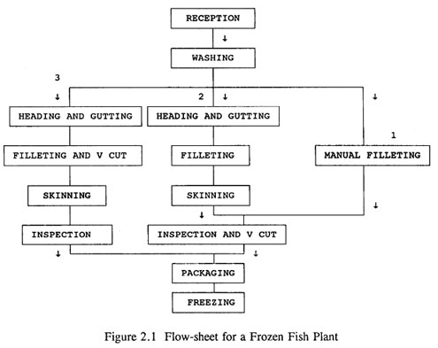
Hake fillets can be prepared manually or mechanically. In the first instance, the same worker heads and guts the fish, separating and skinning both fillets (Line 1). In the mechanical process the following equipment is needed: heading and gutting, filleting and skinning machines.
The machine-made fillet normally has to undergo two manual operations before it is completed. The first, which can be termed enhancing, is a quick procedure and consists of trimming off the black parts (rests of the skin and epithelium) still adhering to the fillet. The result of this operation is a boned fillet. Another operation can be performed along with inspection, which requires more attention from the worker. This entails a complete boning (V-cut) in order to attain a boneless fillet (Lines 2 and 3). As shown in the flow-sheet, the different lines have operations in common.
It should be mentioned that there are machines on the market that perform V-cut automatically, as a continuation of the mechanical line described above, or as part of the filleting process. After a technical and economic evaluation of the different alternatives for manual plants or plants with different levels of mechanization (e.g., 25%, 50%, 75% and 100%), the type of plant can be selected.
A study of frozen fish blocks plants in Argentina has shown that manual processing is better suited for plants with a daily capacity of less than 20 t raw material, and mechanized processing for plants above this capacity (Zugarramurdi and Parin, 1988).
(b) Equipment Selection and Specification
The following equipment is required for the frozen fish plant:
Whole fish weighing machine
Whole fish washer
Sorting table, 2 positions
Filleting table, 15 positions
Inspection and trimming table, 5 positions
Fillet packaging table, 3 positions
Scale Fish block weighing table
Fish block packaging table, 3 positions
Strapping machine
Conveyor belts
Tray washer
Box washer
Tray remover
Freezing trays
Plastic boxes
Fork-lift truck
The number of positions to be filled for each operation is determined from a labour evaluation (see Example 2.13).
Refrigeration equipment:
Blast freezer: 5 t/24 h (*) Plate freezer: 500 kg/load Chill room 0° C: 20 t raw material Cold storage - 30° C: 60 t finished product (FP) Ice-making equipment, capacity: 3-4 t of ice/24 h Ice storage, capacity: 2-3 production days
(*) Note: in practice, it is usual to include a blast freezer, in order to diversify the type of products that could be frozen, for example, headed and gutted (H&G) fish
Ice-making equipment is not indispensable if ice can be bought at a reasonable price, and if continuous supply is guaranteed. This decision depends on an economic analysis of the investment necessary for an internal supply and the cost for purchasing ice.
Example 2.2 Flow-sheet for a Small-scale Tuna Canning Plant
Draw a flow-sheet for a fish canning plant with a daily capacity of 2 670 cans of tuna. Tuna fish canned in oil will be produced, using 180 g cans, with 16% covering liquid. Data for this example are taken from a small tuna canning plant in Cape Verde (FAO, 1986b).
(a) Description of the process
(b) Equipment selection and specification
Answer: (a) Figure 2.2 shows a flow-sheet for a small scale Tuna Canning Plant.
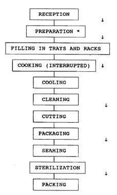
* If using frozen raw material, preparation includes thawing, heading and cutting off the tail
Flow-sheet for a Fish Canning Plant
The number of stages, or their order within the canning process, can vary according to whether large or small species are being used, whether continuous or batch processes have been chosen, whether manual or mechanical labour is being utilized, etc., but at any rate, a standard packaging process can be identified.
The fish is received and unloaded in the plant by electric winches, washed, put in brine, and transported to the heading, gutting and cutting machines. The need for cutting depends on the size of the fish.
Later, the fish is washed again and salted in brine, and finally taken to the processing area. In some industrial plants, salting is achieved by adding salt directly to the can before seaming. In the processing area, there are two possible methods by which the fish can be cooked:
Method I Canned raw and later cooked in the can (still open)
Method II Cooked, cooled, cleaned and canned
Once this stage is finished, oil is added (and salt as necessary) and the cans are sealed by automatic seaming machines. Finally, the sealed cans are sterilized in special retorts, labelled and stored in boxes until distribution.
Technological variables such as salting conditions, duration and temperature of precooking, time and temperature of sterilization, etc., must be chosen according to the species to be processed and the final product, in order to determine the most appropriate process (Parin and Zugarramurdi, 1987). In processing tuna, modifications are made to this general plan. In the current example, Method 11 is used and the tuna is cooked in brine. Later the tuna is cleaned, removing the skin, bones, and red or dark muscle parts, leaving chunks and flakes of tuna. The rest of the operations are the same. When raw material is fresh, preparation includes heading and gutting, and cutting off the tail.
(b) Equipment Selection and Specifications of the Tuna Canning Plant
Reception: 1 crane Weighing: one 0.5 t scale Washing: one 2 000 l tank Heading and gutting: 1 large table and saw Washing: 1 tank Cutting: 1 large table and saw Washing: 1 tank Placing on trays: 1 large table Cooking capacity: 20 trays with 40 kg capacity Transport: 1 crane and two tray carriers Cooking: 1 insulated container Cleaning of cooked fish: 1 large table for two workers Packaging: 1 large table Filling with oil and seal: 1 seaming machine: 10 cans/min Sterilization: 1 retort: 700 cans/load Labelling: 1 large table Boiler: 2 50 kg steam/h
Estimates of this input can be made by working out the quantities of raw material (fish, oil, ingredients, etc.) needed to make one unit of the product. It is important to know if any by-products will be generated by this process.
With the current situation of world fisheries, yield analysis is of paramount importance to fish processing companies. In high valued products, e.g., lobster and shrimp, relatively modest increases in yield lead to substantive increases in profits. In the same way, there is the tendency to improve fish handling and processing to increase yields in commodity products. For instance, the yield in cod processing in Iceland increased by 20-26% in the period 1965-1991 (Valdimarsson, 1992). A comprehensive review of yield and nutritional value of the commercially more important fish species of the world has been published by FAO (Torry Research Station, 1989).
Table 2.1 shows the yield from fish and shellfish which are used as raw materials in the production of different fishery products. Table 2.2 shows the fish net content in different products.
Table 2.1 Yield of Different Species of Fish and Shellfish (1)
Type of Product |
Yield (%) |
Country |
References |
Canned |
|||
Sardines (Engraulis anchoita) |
40-45 |
Argentina |
(Cerbini & Zugarramurdi,1981a) |
Mackerel (Scomberjaponicus marplatensis) |
30-35 |
Argentina |
(Parin & Zugarrainurdi,1987) |
Atlantic bonito (Sarda sarda) |
35-45 |
Argentina |
(Parin & Zugarrainurdi,1987) |
Hake (Merluccius hubbsi) |
38-40 |
Argentina |
(Parin & Zugarramurdi,1986a) |
Tuna (Thunnus spp.) |
50-55 |
Norway |
(Myrseth, 1985) |
Tuna (Thunnus spp.) |
40-44 |
Tropical Countries |
(Edwards el al., 1981) |
Tuna (Thinness albacares) |
38-40 |
Indonesia |
(Bromiley et al., 1973) |
Tuna (Katsuwonus pelamis) |
40 |
Cape Verde |
(1990) |
Shrimp (Penaeus and Metapenaeus spp.) |
28 |
Tropical Countries |
(Edwards el al., 1981) |
Shrimp (Pandalus borealis) |
25-30 |
Norway |
(Myrseth, 1985) |
Frozen |
|||
Hake (Merluccius hubbsi) |
|||
Operation: |
|||
Headed and gutted (H&G) |
60-65 |
Argentina |
|
Manually filleted (Fillet with skin) |
48-52 |
Argentina |
|
Manually filleted (Skinned fillet) |
40-42 |
Argentina |
|
Mechanically filleted (Skinned fillet) |
31 -33 |
Argentina |
|
Trimmed and V-cut |
85 |
Argentina |
|
Manually filleted (Fillet with skin) |
47 |
Uruguay(2) |
(Kelsen et al., 1981) |
Manually filleted (Skinned fillet) |
45 |
Uruguay(2) |
(Kelsen et al., 1981) |
Mechanically filleted (Skinned fillet) |
46 |
Uruguay(2) |
(Kelsen et al., 1981) |
V-cut |
90-92 |
Uruguay(2) |
(Kelsen et al., 1981) |
Product (by hand): |
|||
Interleaved fillets, 4.54 kg |
39 |
Uruguay(2) |
(Kelsen et al., 1981) |
Interleaved fillets, 2.27 kg with skin |
41 |
Uruguay(2) |
(Kelsen et al., 1981) |
Fillet block |
39 |
Uruguay(2) |
(Kelsen et al., 1981) |
Fillet block |
34-36 |
Argentina |
|
White croaker (Micropogonias opercularis) (H&G) |
50-55 |
Uruguay (2) |
(Kelsen et al., 1981) |
Whole white croaker |
97 |
Uruguay (2) |
(Kelsen et al., 1981) |
Striped weakfish (Cynoscion striatus) |
|||
Fillet with skin |
40 |
Uruguay (2) |
(Kelsen et al., 1981) |
Product (by machine): |
|||
Fillet blocks, fatless, 7.5 kg |
37 |
Uruguay (2) |
(Kelsen et al., 1981) |
Fillet blocks, standard, 7.5 kg |
40 |
Uruguay (2) |
(Kelsen et al., 1981) |
Kingelip (Genypterus blacodes) (H&G) |
57-61 |
Argentina |
|
Kingclip (Genypterus blacodes) |
|||
Skinned fillet |
34-40 |
Argentina |
|
Sea Salmon (Pinguipes spp.) (H&G) |
55-58 |
Argentina |
|
Prawn (Pleoticus muelleri argentine) |
|||
Raw, headless |
60 |
Argentina |
|
Raw, headless, skinned |
45 |
Argentina |
|
Shrimp (Pandalus borealis) |
|||
Raw, whole |
95 |
UK |
(Graham, 1984) |
Raw, headless |
60 |
UK |
(Graham, 1984) |
Squid (Illex argentinus) (Gutted, skinned) |
|||
22-44 cm |
72 |
Argentina |
|
49-62 cm |
66 |
Argentina |
|
Cod (Gadus morhua) Skinned fillet |
31.7-39.4 |
Canada |
(Mensinkai, 1967) |
Gallineta (Sebastes mentella) Skinned fillet |
24.0-31.3 |
Canada |
(Mensinkai, 1967) |
Haddock (Melanogrammus aegiefinus) |
|||
Fillet with skin |
36.8-43.7 |
Canada |
(Mensinkai, 1967) |
Sole (Hippoglossoides platessoides) |
|||
Skinned fillet |
21.6-26.0 |
Canada |
(Mensinkai, 1967) |
King crab (Paralithodes camchatica) (Manually processed) |
|||
Operation: |
|||
Batch cooking |
95 |
Canada |
(Amaria, 1974) |
Continuous washing and cooking |
87.74 |
Canada |
(Amaria, 1974) |
Shell removal |
66.25 |
Canada |
(Amaria, 1974) |
Meat separation |
100 |
Canada |
(Amaria, 1974) |
Total yield: |
58.13 |
Canada |
(Amaria, 1974) |
Smoked |
|||
Jack mackerel (Trachurus murphii) |
|||
Filleted |
70 |
Chile |
(FAO, 1986a) |
Smoked |
55 |
Chile |
(FAO, 1986a) |
Total yield: |
38.5 |
Chile |
(FAO, 1986a) |
Biological Silage |
|||
Whole fish and offal (liquid product) |
117 |
Uruguay |
(Bertullo et al., 1992) |
" |
135 |
Venezuela |
(Bello et al., 1992) |
Hydrolysed (Dry Product) |
|||
Enzymatic, human consumption (Humidity: 6%) |
8 |
Cuba |
(Rodriguez et al., 1989) |
Biological (from Merluccius gayi offal) |
12 |
Chile |
(Bertullo, 1989) |
Dehydrated Fishery Product |
|||
FPC (+5% from by-products: oil) |
20 |
Senegal |
(Vaaland & Piyarat, 1982) |
Fishmeal |
25 |
Brazil |
(Vaaland & Piyarat, 1982) |
Rolled dried fish (from minced fish) |
20 |
Brazil |
(Vaaland & Piyarat, 1982) |
Minced fish (from whole fish) |
40 |
Brazil |
(Vaaland & Piyarat, 1982) |
Mechanically and manually dried fish |
31 |
Brazil |
(Vaaland & Piyarat, 1982) |
Naturally dried and smoked |
27 |
Brazil |
(Vaaland & Piyarat, 1982) |
Fishmeal, sun-dried (tuna offal) |
14 |
Indonesia |
(Bromiley et al. 1973) |
Wet Salted |
|||
Anchovy (Engraulis anchoita) |
|||
Headed and gutted |
75 |
Argentina |
(Lupin et al., 1978) |
Salted and cured |
45-50 |
Argentina |
(Lupin et al., 1978) |
Anchovy (Engraulis mordax) |
|||
Headed and gutted |
88 |
Mexico |
(Perovic, 1990) |
Salted and cured |
44.7 |
Mexico |
(Perovic, 1990) |
Mackerel (Scomberjaponicus inarplatensis) |
|||
Cut (60%) and salted (80%) |
48 |
Argentina |
|
Jack mackerel (Trachurus murphyi) and Spanish sardine (Sardina pilchardus) |
|||
Salted and pressed minced fish (humidity: 48%) |
25-30 |
Chile |
(Toro Guerra, 1989) |
Notes:
(1) For more data see Torry Research Station (1989)
(2) Ideal standard yield, based on well handled raw material
Values in Tables 2.1 and 2.2 are only indicative. Yield and fish net content in actual products and actual plants may differ. For instance, in comparing the yield of hake from plants in Argentina and Uruguay, it should be noted that values listed in the table for Argentina were taken from operational industrial plants. Figures given for Uruguay would only be attained if high quality raw material were processed by trained workers. It is possible to achieve an improved yield of products based on hake fillets; and in Uruguay, according to Kelsen et al. (1981), a 6-7% increase could be achieved.
Table 2.2 Fish Net Content in Different Products
Type of Product |
Net Content (%) |
Country |
References |
Battered and Breaded Products |
|||
Meat content in product (%) |
|||
Breaded shrimp |
52 |
India |
(Pedraja, 1987) |
Pre-fried breaded clams |
56 |
" |
" |
Pre-fried breaded squid |
35 |
" |
" |
Cooked shrimp burgers |
46 |
" | " |
Cooked shrimp yield |
72 |
" |
" |
Tuna burgers |
|
||
Thin |
53 |
" |
" |
Large |
46 |
" |
" |
Fish sticks |
41 |
" |
" |
Skinned, boneless, cooked tuna yield |
80 |
" |
" |
Shark burgers |
|||
Thin |
44.5 |
" |
" |
Fish sticks |
41.6 |
" |
" |
Cooked shark yield |
87 |
" |
" |
Pre-fried, battered, stuffed squid tubes |
50 |
" |
" |
Breaded hake fillet |
80 |
Argentina |
|
Prepared Foods |
|||
Tuna in tomato sauce |
47.6 |
India |
(Pedraja, 1987) |
Shrimp in tomato sauce |
52.5 |
" |
" |
Canned |
|
||
Sardines (Engraulis anchoila) 170 g ea |
75-80 |
Argentina |
(Parin & Zugarramurdi, 1987) |
Sardines (Clupea pilchardus) 125 g ea |
72 |
Tropical countries |
(Edwards et al., 1981) |
Sardines 125 g ea |
76 |
Norway |
(Myrseth, 1985) |
Herrings 195 g ea |
67 |
" |
" |
Mackerel, 195 or 250 g ea |
67-72 |
" |
" |
Shrimp, 111 or 217 g ea |
67-69 |
" |
" |
Tuna, 12 r 200 g ea |
76-77.5 |
" |
" |
Fish cakes, 400 or 800 g ea |
65 |
" |
" |
Sardines, 125 g ea |
72 |
Tropical countries |
(Edwards et al., 1981) |
Shrimp, 200 g ea |
64 |
" |
" |
The yield of each operation and the final production yield must be known. It is also important to know how yield varies according to the quality of raw material, the training of the worker, size of the fish, change in the sequence of operations, etc. Published results indicate that the raw material yield diminishes when there is a lack of: quick icing onboard (10-15%) and sorting (7%). In the case of fish near the acceptability limit, the yield reduction could be up to 25% (e.g., anchovies for fish salting). Raw material quality has a great impact, since in addition to the decrease in yield it increases labour and in practice reduces production capacity (Montaner et al., 1994a). Actual yields should be researched in each plant. Table 2.3 shows the yield values for production of interleaved hake blocks according to quality of raw material and worker training (from Kelsen et al., 1981).
Table 2.3 Final Yield by Quality of Raw Material and Worker Training
Quality of raw material |
Good |
Good |
Average |
Average |
Worker training |
Good |
Average |
Good |
Average |
Final yield (%) |
39.3 |
34.7 |
36.5 |
32.2 |
If an operation performance is defined as the variation in yield for good or average quality raw material over highest yield, it will decline by 7%, whereas if both quality and training are considered, the value increases to 18%. Table 2.4 shows that the highest yield is achieved when sorting is done before processing (from Kelsen et al., 1981).
Table 2.4 Overall Yield of Frozen Unglazed Mechanically H&G Croaker (M. opercularis). Effect of Sorting by Size
Yield (%) |
With sorting |
Without sorting |
Actual |
48 |
44.3 |
Ideal |
50-55 |
- |
*Based on quality and handling of raw material
Given the high percentage of the cost of raw material in the final production costs, all recommendations for the treatment of raw material must be considered in order to maintain the initial quality of the fish. It is essential that the FIFO principle (first in, first out) be applied, rigorously controlling the order in which raw materials are processed, in order to achieve a high final yield. Finally, Table 2.5 shows the use of other raw materials such as salt, oil, etc., in the production of fishery products.
Table 2.5 Consumption of Various Raw Materials in the Production of Fishery Products
Type of Product |
Consumption |
Country |
Reference |
Battered and breaded products |
|||
Tuna burgers |
|||
Bread |
12-31 % of product weight |
India |
(Pedraja, 1987) |
Stuffed squid |
|||
Battered and pre-fried |
|||
Stuffing |
30% of product weight |
India |
(Pedraja, 1987) |
Batter |
20% of product weight |
" |
" |
Smoked yellow jack mackerel |
|
||
Salt |
0.1 kg/kg of fresh fish |
Chile |
(FAO, 1986a) |
Sugar |
0.07 g/kg of fresh fish |
" |
" |
Canned |
|||
Oil |
0.1 kg oil/kg sardine raw material |
Argentina |
(Parin & Zugarramurdi, 1987) |
| 0.25 kg oil/kg final product | " |
" |
|
Salt |
0.012 kg salt/kg of whole sardine |
" |
" |
| 0.03 kg salt/kg of sardine final product | " |
" |
Example 2.3 Raw Material Requirements
Calculate the consumption of raw material for the frozen fish plant in Example 2. 1. The raw material is whole hake.
Answer: To determine the quantity of raw material required for obtaining 2 t of finished, skinned, hake fillet, all that needs to be known is the total yield of the operation. Table 2.1 shows that the yield for manual production of skinned, boned, frozen hake varies between 34 and 36%.
Raw Material Required
(t) = Plant Capacity in Finished Product / Yield (decimal)
(t) = 2 t of fillets / 0.34 (t whole/t fillets) = 5.9 t
Thus, 5.9 t of whole hake will be required to produce 2 t of skinned fillets.
Knowing the yield of each operation is useful to compare actual yield with theoretical yield and assess how efficient the operation is or to discover what or where the losses are. When the yield of different stages of processing is analysed, calculations can be more complicated, as the basis for calculation varies. An example follows:
Example 2.4 Raw Material Requirements, by stage
Calculate the consumption of raw material, at each stage, filleting, trimming', and V-cut for the frozen fish plant using manual processing, described in Example 2. 1. The raw material is whole hake.
Answer: Generally, the results are expressed in terms of units of finished product (in this case 1 kg of finished fillet). This value is obtained by multiplying the weight (kg) of the product at each stage by the yield of the stages which have not yet been completed.
Graphic representation of the effect of the processing of fish:
Whole hake Filleted Trimmed 1000 g Q 400 g Q 340 g The 5.9 t of whole raw material gives a yield of 34% when filleted.
5.9 t raw material x 0.4 = 2.36 t of fillets (un-trimmed)
2.36 t of fillet x 0.85 = 2 t of finished product (skinned, boned fillets)
Overall yield 0.4 x 0.85 0.34 (or 34%)
Example 2.5 Raw Material and Input Requirements
Calculate the use of raw material for the fish canning plant in Example 2.2. The raw material is tuna.
Answer:
Fish: To calculate the quantity of fish required for daily production of 2 670 cans, the following formula will be used:
Daily Production (cans/day) x Net weight (kg/can) x (1 - filling, expressed as a decimal) /Total yield (decimal)
= 2 670 cans/day x 0. 180 kg/can x (1 - 0. 16) / 0.4 = 1 009 kg raw material/day or approximately 1 000 kg raw material/day
(filling: oil, brine or sauce added to canned fish during processing)
Oil: Daily production (cans/day) x Net weight(kg/can) x Filling expressed as a decimal =
2 670 cans/day x 0. 180 kg/can x 0. 16 = 77 kg oil/day approximately 80 kg oil/day
This calculation is the exact quantity that must be added to the can. During actual plant operations, however, a greater quantity is consumed, usually 1-2%, due to losses.
Salt: Daily production (cans/day) x Fish content (kg/can) x (1- filling expressed as a decimal) x Salt expressed as a decimal = 2 670 cans/day x 0.180 kg/can x (1-0.16) x 0.03 = 12 kg salt/day
Thus, 1 t of tuna, 80 kg of oil and 12 kg of salt will have to be utilized daily in order to produce 2 670 180~g cans of tuna in oil per day.
The values in Tables 2.1 to 2.5 and other tables with numerical values which appear in the text, must be taken as illustrative values, to serve as guides in a first analysis of the processes. It is clear from analysing these tables that in practice there are variations in the values published by different authors. These variations are due to diverse causes that the technologist must be able to identify in each specific case, and which generally pass unnoticed in common economic analyses. The authors opine that widespread and indiscriminate use of factors in calculating yield and inputs is one of the reasons for the failure of undertakings in this area.
The following example analyses causes for variation in use of salt in fish salting.
Example 2.6 Technical Analysis of the Use of Salt in Fish Salting
Make a technical analysis of the use of salt in fish salting
Answer: Only a certain quantity of salt can be absorbed by fish flesh. At saturation, this quantity is equal to the amount of salt that would dissolve in a quantity of water equal to what the fish might have at the moment of establishing equilibrium; that is, the salt is mainly forming a brine, of the same concentration as can be found outside the fish, inside the fish flesh.
The flesh cannot absorb solid salt (Zugarramurdi and Lupin, 1976, 1977). From this, it is possible to calculate the minimum quantity theoretically needed to salt fish. For example, for salting anchovies and other small pelagics, Mediterranean style (headed and gutted fish, simple or butterfly fillets, wet salted, with pressure, for a product with a water activity value of 0. 75), the quantity of salt required can be estimated at 20-25 % of the total fish weight to be salted (variation is due to the lipid content). This minimum quantity is generally not recommended, since it is desirable for the container to have an excess of salt.
The excess salt in the bottom of the salt barrel guarantees that the fish has been saturated with salt (a control for the process). Thus, in practice, a higher percentage of salt, 30-40% of total fish weight, is recommended for this process (Lupin, Zugarramurdi and Boeri, 1978). From the point of view of inputs, this quantity can be greater due to other factors such as quality or coarseness of the salt or a different salting process.
If the salt is impure and dirty, as happens with many solar produced salts in developing countries (salt produced directly from the action of the sun on seawater), the salt must be washed before it is used for salting fish (washing with tap water is sufficient to eliminate substances such as sand, reduce the content of other salts and also reduce level of contamination by halophilic bacteria). Depending on the intensity of washing, 10-20% more salt may have to be used.
If the process is dry salting (i.e., accumulated brine is drained), more salt is added so as not to risk spoilage due to insufficient salt. It is not easy to estimate this quantity, as it depends on the coarseness of the salt and other factors such as type and shape of fish to be salted. If the available salt is very fine (crystal size of 0.5-1.5 mm) brine drainage will take a large quantity of the salt with it. If the salt used is of a larger grain (more than 3-5 mm) a larger quantity of salt will be required to ensure that the various layers of fish in tile dry stack are covered with salt. For best results (one-third fine crystals to ensure rapid brine formation on the fish and two-thirds crystals of 3-5 mm size to maintain brine saturation), an estimated 20-30% more salt will be needed for the dry-salting process.
In calculating total inputs, account must be taken of salt losses incurred in transportation and storage. These losses are obviously related to the quantity of salt used, care in handling and storage, etc. Losses can be estimated at approximately 10%.
Salt content in the final product will depend largely on the pressure. Products which are wet salted without pressure weigh more when finished, and their brine content (and therefore salt content) is greater than those wet salted with pressure. Products which are wet-salted without pressure will require additional salt.
It can be estimated, for example, that a wet-salting process using pressure, where the salt needs to be washed, will require a quantity of salt equivalent to 50-70% of the total weight of the fish already prepared for salting. If it is desirable to relate this quantity to raw material, and assuming a yield of 75%, between 37 and 52% of the weight of the raw material will be required in salt.
It could be argued that in practice, the cost of salt could have little influence on total cost, and that a detailed analysis would therefore not serve any real purpose. This could be the case, for example, with the salting of cod in North European countries. However, there are countries and types of exploitation where the cost of salt is a major and significant input.
The authors have found that salt cost can rise to US$ 1-2/kg in remote islands (in Asia and in the South Pacific) and in the interior of Africa when transport difficulties exist. For instance, an FAO project carried out in the Maldives demonstrated that the only economically viable possibility for fishermen located in islands far from the capital, to produce salted fish, was to produce their own salt.
In short, analysing inputs must be considered in reference to a particular process, in a specific area or country, and within a general cost structure.
A summary of this analysis is shown in Table 2.6.
Table 2.6 Technical Analysis of Salt Consumption
Process |
% of salt needed (kg salt/kg fish to be salted) |
Wet salted |
|
- with pressure |
30-40 |
- without pressure |
40-50 |
Dry salted |
|
- normal |
50-60 |
Salt washing |
10-20 |
Losses |
10 |
The previous example illustrates the difficulties in making a technical analysis of a process as simple as salting. The analysis of an input at the industrial level is, in practice, more complex.
The amount of ice required to chill and store chilled fish depends on several factors, and there is no immediate rule to calculate it. However, when the situation is repeated every day, when it is necessary to purchase an ice plant, to calculate a chilled fish distribution chain or to furnish ice to a fleet, an accurate calculation of the ice requirements must be made.
Common fish handling advice is usually based on the use of concepts like "plenty of ice" and "re-icing". The simple rules found in many technical publications are matters of discussion in many practical situations. Moreover the economic impact of the cost of icing fish (cost of ice plus quantity required) in developing countries is different from that in developed countries where it can be considered negligible.
The ice consumption icing fish can be divided into three terms:
Total ice consumption |
= |
Ice necessary to cool fish 0°C |
+ |
Ice melted to compensate for thermal losses |
+ |
Ice handling losses |
(2.1) |
The division in different terms is useful to evaluate the extent and weight of the losses.
The ice necessary to cool fish to 0°C can be calculated theoretically, i.e.
(2.2)
where:
Cpf = specific heat of fish (kcal/kg °C), the cpf varies with the composition, it will be around 0.80 kcal/kg °C for lean fish, 0.78 kcal/kg °C for medium fatty fish and 0.75 kcal/kg °C for fatty fish
Tf = fish temperature (°C), usually taken as the sea water temperature
= latent heat of fusion of ice (kcal/kg), usually taken as 80 kcal/kg
Mf = mass of fish
If all the factors are put together in Equation (2.2) the following equation is obtained for lean fish:
(2.3)
or
(2.4)
Equation (2.4) can be taken as a quick approximate way to calculate the amount of ice to cool down fish to 0 °C (in all the other cases the required amount of ice will be lower than such required for lean fish). For example, if fish caught is at 25°C, the result will be 0,25 kg ice/kg fish. Why in practice is much more ice necessary?
The general answer is to compensate for losses; the most important losses are thermal. Ice is utilized to cool down fish to 0 °C, and in doing so, ice melts. Ice melting rates, due to thermal losses, depend mainly on external temperature and the type of container where the iced fish is stored (in particular the insulation characteristics of the container's walls, and its geometry). It can also depend on how and where the fish boxes or containers are stacked. In general the equation that relates the ice melted to compensate for thermal losses will be:
(2.5)
or
(2.6)
where:
Mi(t) = mass of ice in the box/container at time t (kg)
Mi(0) = initial mass of ice in the box/container at time t = 0 (kg)
= average external temperature (°C)
t = time elapsed since icing (hours)
k = specific ice melting rate of the box/container [kg of ice] / [hour x °C]
The k value can be very easily determined
experimentally in boxes (Boeri et al., 1985) and insulated
containers (Lupin, 1985a). In principle it could be determined
theoretically from the box/container thermal characteristics;
however, in practice, wide variations can be found due to the lid
type, drainage and to a lesser extent due to the type of ice and
the actual volume occupied by fish and ice in the box/container.
The experimental determination of k is advised particularly when
large volumes of ice are utilized. In actual conditions the
external temperature (![]() ) fluctuates. However, acceptable calculations are
obtained assuming an average temperature (
) fluctuates. However, acceptable calculations are
obtained assuming an average temperature (![]() ), from the beginning until the end of the
specific storage trial. In this case, the following relationship
can be defined:
), from the beginning until the end of the
specific storage trial. In this case, the following relationship
can be defined:
For example, the values of k and k' for two types of fish containers are as follows:
(i) Standard plastic box (polyethylene, 40 kg, Boeri et al., 1985)
k = 0.22 (kg of ice/day x 0 °C)
k' = 0.22 x
(ii) Insulated container (Metabox 70 DK, Lupin, 1985a)
k = 0. 108 (kg of ice/day x 0 °C)
k' = - 0.04 + 0.108
Ice stored at ambient temperature has a certain amount of water on its surface: this means that when ice is weighed a certain part of the weight is already water. The larger the ice surface per unit of volume, the higher the amount of water in equilibrium. The amount of water in equilibrium in sub-cooled ice is nil (the ice sticks to the fingers), and in ice bars is negligible. However, in all the other types of ice stored above 0°C, it has a value. In Table 2.7 the measured amount of water in equilibrium for different types of ice is shown:
Table 2.7 Average Percentage of Water in Equilibrium in Different Types of Ice, Stored at 27 °C (Boeri et al., 1985)
Ice type |
Equilibrium water (% wt/wt) |
Flake ice |
12- 16 |
Crushed block ice |
10- 14 |
Ice chips |
16-20 |
Additional losses are due to bad handling and melted water in equilibrium over the ice surface. Losses due to bad handling (e.g., ice fallen on the floor or thrown away when ice in boxes or containers is levelled) are very difficult to assess since they depend on many factors (including worker's skill), but they are probably not lower than 3-5 % of the amount of ice utilized. Apart from the effect on the economic performance this type of loss should be reduced as much as possible for reasons of hygiene and working safety.
All calculations on ice consumptions should be made on a weight basis, since different types of ice have different volumes for the same weight, and the cooling capacity (latent heat of fusion of ice) is expressed in kcal/kg. Water from melted ice, even at 0°C, has a negligible cooling effect on fish (it is useful for other purposes, e.g., to improve heat transfer, to keep the fish moist).
A consolidated picture of the different ice requirements is given in Table 2.8.
Table 2.8 Some Values of Ice Required for Icing Fish
Ice necessary (kg), or (kg/day) |
|||||||
Consumption/loss factor |
|
Ref. |
|||||
1 |
2 |
5 |
10 |
20 |
30 |
||
- To cool down 1 kg of fish to 0 °C |
0.01 |
0.03 |
0.05 |
0.10 |
0.20 |
0.30 |
Eq. (2.4) |
- To compensate for thermal losses (in kg/day for a given box/container) |
|||||||
Examples |
|||||||
i) Standard plastic box (40 kg) (Boeri et al., 1985) (1) |
0.22 |
0.44 |
1.1 |
- |
- |
- |
Eq. (2.7) |
ii) Insulated container (Metabox 70) (Lupin, 1985a) |
0.068 |
0.176 |
0.5 |
1.04 |
2.12 |
3.2 |
Eq. (2.8) |
Ice necessary as % of the initial mass |
|||||||
- To compensate for bad ice handling |
3-5(2) |
||||||
- To compensate for water in equilibrium |
12-20(3) |
Table 2.7 |
|||||
Notes:
(1) Experiments were carried out only between 0°C
and 5°C, values correspond to a box stacked in the middle of a
stack
(2) Minimum estimated values
(3) Depends on type of ice and storage temperature
It is interesting to analyse results for ![]() from 1 °C to 5 °C in
Table 2.8 to assess ice consumption when a chill storage room (or
chill storage hold) is utilized, and values of
from 1 °C to 5 °C in
Table 2.8 to assess ice consumption when a chill storage room (or
chill storage hold) is utilized, and values of ![]() from 10 °C to 30 °C
to analyse when iced fish is stored/transported at ambient
temperature in standard boxes or insulated containers,
particularly in tropical conditions.
from 10 °C to 30 °C
to analyse when iced fish is stored/transported at ambient
temperature in standard boxes or insulated containers,
particularly in tropical conditions.
A wide variety of situations exists and the recipes (e.g., "use 1:1 ratio", "use 1:2 ratio") are, therefore, meaningless. This type of recipe is at the root of many past failures when attempting to introduce ice in artisanal fisheries in tropical developing countries, because they may lead to technical and economic mistakes. A systematic approach for the ice consumption in insulated containers is available in the literature (Lupin, 1985b); however, approximate estimations can be made from the data in Table 2.8 (for other types of boxes/containers, the experimental determination of k is advised).
In practice, a ratio fish to ice (or ice to fish) is defined as follows:
Mf / Mi° = n (2.9), or: Mf = n x Mi° (2. 10)
Also, as a container has a finite volume, the following relationship holds at t = 0, assuming the container is completely full:
Vc = Mf x Vsf + Mi° x Vsi (2.11)
where:
Vc internal (utilizable) volume of the container (cm3)
Vsf specific volume of fish stowed (cm3/kg)
Vsi specific volume of ice stowed (cm3/kg)
In the experiments mentioned by Lupin (1985a), the values of Vsf and Vsi are:
Vsf 1274 cm3/kg (barracuda Sphyraena spp., Tanzania)
Vsi 1731 cm3/kg (flake ice)
It should be said that Vsf and Vsi can easily be determined in actual conditions by weighing a known volume of fish or ice. In order to determine how long ice will last in the container, some of the above relationships may be rearranged to obtain the time that is necessary to keep the mixture of fish and ice (tMAX), which is usually fixed by the conditions of storage and transport. It is possible to define a t*MAX when no fish are in the container and all the ice is used to compensate heat losses. In this case:
(2.12)
All the above expressions can be rearranged to:
(2.13)
Equation (2.13) is represented in Figure 2.3 for three different fish temperatures.
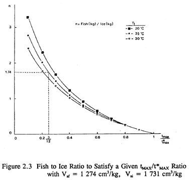
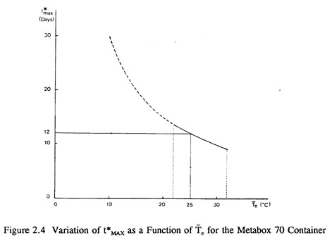
On the other hand, t*MAX can be represented as a function of Te for a given type of container, using expression (2.12). This equation is represented in Figure 2.4 for the Metabox 70 container (Lupin, 1985a). Figure 2.4 can be determined after an evaluation of the thermal effectiveness of the container (Lupin, 1985a).
It is important to discuss ice consumption, particularly in developing countries. As will be seen later, 1 kg of ice can, in many places, represent a significant proportion of the cost of 1 kg of fish and is sometimes even more expensive.
Example 2.7 Introducing Plastic Boxes in Artisanal Fisheries
Fish is plentiful near the islands off the coast of Ruritania; however, it takes up to six hours for iced fish to arrive from the island villages to the capital city where a growing fish market exists. Ice is available in the capital city and arrangements can be made to return the fish boxes (after washing) full of ice. Plastic boxes were recommended because they were found more hygienic than local wooden boxes (public officers are concerned about public health aspects).
Average temperature in Ruritania is around 30 °C. It was suggested to utilize standard plastic boxes covered by a tarpaulin to do the job. Do you think it is feasible?
Answer: As recommended in section 2.4.2, an experimental determination of ice consumption was carried out in order to obtain reliable results at the expected working temperatures. The results are presented in Table 2.9 Table 2.9 Ice Consumption in Plastic Boxes in the Tropics (1)
Box type |
Storage |
|
k (kg ice/hour) |
- with drainage (2) |
Shade |
28 |
1.13 |
Sunshine |
30.4 |
3.12 |
|
- without drainage |
Shade |
28 |
2.13 |
Sunshine |
30.4 |
5.30 |
Notes:
Actual experiments were conducted at the FAO/DANIDA Workshop, Guinea-Bissau 1986, with plastic boxes of about 35 kg (of water) capacity each. Full flake ice capacity about 20 kg. Measurements done on individual (not stacked) boxes.
Water retained in the box allows for better heat transfer and therefore increases the ice melting rate.
There may be an influence of radiation in the case of boxes exposed to sunshine.
From Table 2.9, it is possible to deduce the following:
Plastic boxes without the coverage of a tarpaulin (shade) cannot be utilized since exposure to sunshine increases dramatically the ice melting rate (around 160% over the ice consumption in the shade) and, in any case, ice will be melted before it arrives on the islands.
Plastic boxes without drainage showed, in this case, an increased ice consumption even in the shade and in the best of cases, only a reduced fraction of the initial amount of ice in each box (about 13 kg per box) will arrive on the islands.
About 10 kg of fish could be fitted in each box (almost the 1: 1 ratio). Chilling the 10 kg of fish will take around 3 kg of ice, and the journey back to the capital will consume a little less than 7 additional kg of ice. In principle, there are still 3 kg of ice per box left to provide for loading and unloading time and unexpected delays and other losses.
However, the risks of delays should be carefully assessed and the economics of utilizing 2 kg of ice to transport 1 kg of fish should be analysed before taking a decision. Moreover, if fish is to remain overnight in the capital city (and this is a possibility) before being sold the following day, it will be necessary to re-ice the fish a couple of times and total ice consumption will rise to 4 or 5 kg/kg of fish and ice costs will become prohibitive. In most cases, unless an expensive product is involved (e.g., shrimp), this procedure will not be viable and another solution must be sought.
Example 2.8 Introducing Insulated Fish Containers in Artisanal Fisheries I
The insulated container of Table 2.8 will lose 0.8 kg of ice en route from the town to the village; each container will have a large amount of ice, enough to fill it with fish and reship it back to town. Ice will be sufficient to compensate for other losses that may occur, for instance an overnight wait for the ferryboat early in the morning. As in this case, a proportion of 1 kg of ice per 2 kg of fish will be more than enough to transport fish to town; not all the incoming insulated boxes need be full of ice. However, fishermen may require additional ice to keep fish fresh if not caught a few hours before shipping the fish to town.
This example shows that the introduction of insulated containers could be a sound technical solution. However, it introduces additional costs (ice plus insulated containers) and a type of relationship and coordination between purchaser and buyer that may not exist. In this situation, extension services have a lot of work to do.
Example 2.9 Introducing Insulated Fish Containers in Artisanal Fisheries II
Continuing with the situation described in examples 2.7 and 2.8, it could be assumed that the introduction of insulated containers analysed in 2.8 was initially a success. Local extensionists and foreign technical assistance run a scheme that gave good results, increased the quality and amount of fish shipped to town and the fishermen's income.
At a certain point, the extension service decided to stop the assistance and passed operations onto the fishermen and buyers. Everything was fine for a while until certain problems arose. The first was that the success generated the interest of fishermen in more remote islands in the archipelago and fish was arriving in the village in quantities that required much more ice than before. It was now necessary to reship ice to the most remote islands from the village. At the same time, the system required a coordination and understanding between buyer and seller not always easy to achieve. Sometimes, the ferry did not arrive and this generated fish losses because ice was insufficient to keep all the fish until the next day. Ice and fish storage capacity is now necessary at the village.
The installation of an ice plant and a cold storage room in the main fish village may now be an attractive possibility provided the village has enough electricity; if not, a generator could be installed. In any case, this possibility should be checked out from an economic point of view, to determine if it is self-sustainable.
An alternative transitory solution could be to transport ice bars from the capital city to the village. Ice bars melt slowly and take less volume per unit of ice weight (making transport and storage less bulky). Fishermen could crush the ice just before using it to chill fish. This alternative is used by artisanal fishermen in countries like Colombia, Philippines and Senegal where they have developed the system by trial and error. The ice bar solution gives fishermen a little more flexibility than the flake ice solution and does not require much investment. However, extensionists should study the feasibility of this system carefully, considering time and distance from the market, before they advise it.
There is a second transitory solution: to increase the volume of the insulated containers. As thermal losses are proportional to the area exposed to the air, the increase in volume will reduce the ice losses per 1 kg of fish (and per 1 kg of ice when transported and stored). The drawback of this solution is that insulated containers could become too heavy to move for loading and unloading; at the same time, in large containers there is the risk of fish losses by mechanical damage and lack of proper icing. Despite this limitation, large insulated containers can be found in operation, e.g., in Tanzania and Uganda.
This example could be complicated in different ways, for instance, the ferry company may impose a maximum volume on transport because passengers and other goods should also be transported (not an unlikely situation in some African countries). Development is in practice a continuum of situations, very difficult to assess beforehand. This example shows that a technical solution does not necessarily work forever even if initially successful. The raw material calculation, in this case ice, may be affected for many different reasons, to be specified in each case. Theoretical calculations (application of equations 2.1-2.6) are obvious; therefore, examples 2.8 and 2.9 mainly aim to clarify that determination of actual conditions to which such calculations apply is the first important step.
Example 2.10 Ice and the Fish Quality for a Given Market: the Zero Ice Option
For many years the fishermen in the previous example were sending un-iced fish in artisanal containers to the capital city (they knew which type of fish was suitable). Local customers were waiting for the fish and it can be calculated that the fish was consumed around 10- 12 hours after being caught. It was not the best solution but in the past it worked.
However, the capital city of Ruritania grew considerably and a fish market was organized by the Government. Now the customers can no longer buy directly from the fishermen and have to go to the market. Obviously, it takes considerably longer than before for the fish to reach the customer and, as restaurant owners and fish exporters are also buying fish from the fish market, they complain about the quality of the fish from the islands.
The Government does not want to return to the previous situation and, moreover, wants to enforce rigid hygienic and sanitary regulations to protect public health and exports. The Government fish market was organized to expand the supply, to curb excessive middle man action to benefit both fishermen and consumers, and to improve fish hygiene and quality which were at risk in the former informal market with the increase of fish consumers.
Fishermen do not understand how things changed so suddenly, and this is the situation that generated the proposition discussed in Example 2.7. Imagine you are a Government Fish Extensionist - how could you explain the situation to the fishermen?
Answer: Iced fish is almost synonymous with fresh fish. However, there is a very short period - immediately after catch - during which fresh fish may stay without ice. Fish spoils very quickly but if it is kept moist, in the shade, and away from filth and animals, it keeps its edible quality for some hours; there is no fixed rule on how long since this depends largely on the type of fish. For instance, some small pelagics can develop a large amount of histamine after only 4 or 5 hours of storage at ambient temperature (Ababouch, 1991), but other species - in particular some lean and flatfish - can last longer.
Fishermen know usually from their own experience how long this period can be and they also know that the fish should be consumed as soon as possible and cannot last till the following day in such conditions. However, when additional delays are introduced, or when fish is not consumed right away or needs further processing or when the middle-man chain expands, the picture changes dramatically, since fish in such conditions lose quality which cannot be recovered. Moreover, the fish may become unsuitable for consumption from the health point of view.
The zero ice consumption option works within very narrow time limits and temperatures and is generally the first stage of the fish consumption development pattern. It comprises the subsistence condition and early marketing stages when quick consumption or processing follows landing, very few hours after catching.
Example 2.11 Ice Consumption in a Fish Chill Room
In an industrial plant, fish iced in flake ice is stored in a chill room (average 5 °C) in 40 kg plastic boxes. Normally fish stay in the chill room about 12 hours. The manager wants to know the effect of reducing the temperature of the chill room from 5 °C to 3 °C. Apart from reduction in ice consumption what additional benefits could be expected?
Answer: Following the figures of Table 2.8, the calculations are as follows:
Table 2.10 Ice Losses in a Chill Room
Condition |
Thermal losses in 12 h (kg) |
Ice handling
losses (kg) |
Water in
equilibrium |
Total ice
needed |
Box at 3 °C |
7.92 |
0.32 |
0.95 |
9.10 |
Box at 5 °C |
13.20 |
0.53 |
1.58 |
15.31 |
Thus, reduction of the chill room temperature from 5 °C to 3 °C will mean a reduction in ice requirements of about 40% (the economic convenience of reducing the chill room temperature should be checked independently). The reduction of the amount of ice required means in practice a net increase in the fish storage capacity. The increase in terms of weight depends on the specific volumes (cm3 /kg) of fish and ice stowed in the boxes. Assuming that the specific volume of flake ice is 1731 cm3/kg, and that a small type of fish of 1 300 cm3 /kg is stowed (Lupin, 1985b), a total of 10 593 cm3 will be available per box which, in practice, will allow more than 8 kg of additional fish per box. This is not a negligible amount.
Utilizing the same specific volumes it is possible to calculate that in the 5 °C storage situation, the amount of fish cannot be higher than 10 kg per box (please note that a box of 40 kg will contain 40 kg of water and the weight of ice and fish contained will be much lower). This means that a reduction in the chill room temperature from 5° to 30 °C will give an increase of around 80% in the actual fish chill room capacity.
These results which are known to the well-experienced fish chill room operators are systematically ignored and the ingrained tendency to follow general and untested recipes unfortunately prevails. Whereas this aspect may be of little importance in developed countries (to be verified), they became important in developing countries where there is a need for better ice and fish chill room design and management. However, it is expected that the current trend towards the application of quality assurance concepts that also involve yield, economics and management, as well as fish quality, will subject all fresh fish handling and processing procedures to a more rational analysis.
Example 2.12 Fish to Ice Ratio Calculations
Determine the appropriate fish to ice ratio for a given set of conditions in two different developing tropical countries and compare the results obtained for a temperate developed country. (Real data were compiled by the authors during the FAO/DANIDA Regional and National Training Workshops on Fish Technology and Quality Control.)
Answer: From values in Table 2.11 and equations (2.12) and (2.13), values in Table 2.12 can be obtained.
Table 2.11 Data for Example 2.12
Parameters/Country |
Paraguay |
Trinidad & Tobago |
Denmark |
||
Type of container |
(1) |
(2) |
(3) |
(4) |
(5) |
Vol.cont.(1) |
50 |
100 |
30.7 |
48.52 |
64.8 |
k (kg/day x °C) |
0.0938 |
0.263 |
0.155 |
0.195 |
0.104 |
Te (°C) |
32 |
32 |
31.3 |
28.3 |
10 |
Tf (°C) |
22 |
22 |
25 |
25 |
8 |
Vsi cm3/kg |
1156.07 (6) |
1156.07(6) |
1569.9 (7) |
2060.3(6) |
1731(8) |
cpf kcal/kg x °C |
0.78 |
0.78 |
0.78 |
0.78 |
0.8 |
Vsf cm3/kg |
1858(9) |
1885(10) |
1466.8(11) |
1466.8(11) |
1274(12) |
tMAX (days) |
2 |
2 |
2 |
2 |
3 |
Notes:
(1) Styrofoam box
(2) Metallic, styrofoam insulation
(3) Plastic, styrofoam insulation
(4) Rubber, insulated
(5) Metabox 70 (DK)
(6) Tube ice
(7) Crushed ice
(8) Flake ice
(9) Prochilodus scrofa (characin)
(10) Salminus maxillosus (jaw characin)
(11) Red snapper
(12) white fish
Table 2.12 Results for the Data in Example 2.12
Parameters/Containers |
(1) |
(2) |
(3) |
(4) |
(5) |
t* MAX (days) |
10.67 |
7.61 |
4.03 |
5.60 |
36.00 |
n |
1.57 |
1.16 |
0.71 |
1.32 |
6.4 |
From the results appearing in Table 2. 11, it is clear that it is very difficult to generalize regarding a proper fish ice ratio. Of the cases presented in Table 2.12, only one (case 2) is about the classic option n = 1, in case 3 the option n = 1 will not be enough and, in the other cases n = 1 will be above the specified needs. In extreme cases, it may imply wastage of ice and insulated container capacity.
Although in some modem fishing vessels there are automatic icing devices that can dose ice according to the fish flow, the advice is to look in practice not for the theoretical decimal proportions but for workable proportions (e.g., using gauged buckets or number of shovelfuls) in order to accommodate the amount of ice really needed.
The engineer can find varying degrees of information, ranging from detailed information on the number of workers required per shift (during production) to the complete absence of data.
There is no quick method that can be universally applied to estimate labour requirements. The method of making estimates based on the sequence of production operations is presented. If a flow-sheet for the process or a chart showing the location of equipment in the factory is available, labour requirements can be estimated.
Table 2.13 shows typical direct labour requirements for the fishery industry, expressed as consumption of man-hours per unit of product.
Table 2.23 shows typical manpower requirements (per unit of finished product) and in supervision, for different fish plants. This Table is placed at the end of this chapter because it also contains information on services requirements for different fish processing plants. For some of the processes, the personnel required for management, administration and supervision, are shown in the third column of Table 2.23.
From the analysis of Table 2.23, it can be deduced that fish canning plants, with mechanical heading and gutting operations, producing more than 30 000 cans of 170 g each daily, require an average of 30 workers per t of finished product. This figure increases to more than 60 workers if there is a substantial decrease in plant capacity whereas, in a completely mechanized process, only 8 workers are required.
In fish freezing plants, the average estimate is about 10 workers per ton of finished product. There is a wide ariation in the required number of supervisors, since there are manual and mechanical plants and different levels of technological development (efficient use of manpower and equipment); the highest figure is for manual plants in developing countries. Note should be taken of the low incidence of direct labour in fishmeal plants.
Finally, there is a wide variation in the use of labour per ton of finished product. This depends basically on the type of process used and the capacity of the plant. Totally manual plants, on the other hand, require more than 100 workers which renders large capacity manual fish canning plants non-viable. This short example demonstrates that common sense and experience are necessary to assess labour requirements in practice.
Table 2.13 Typical Direct Labour Requirements in the Fishery Industry
Type of Plant |
Work requirements |
Reference |
|
| Cannin | |||
Argentine Sardines (Engraulis anchoila) |
|||
Manual Process |
Labour, min/100 cans 170 g |
Argentina (Parin et al., 1987b) |
|
Headed and gutted |
22-30 |
" |
|
Put in trays and Cooked |
9- 13 |
" |
|
Packaged |
30-45 |
" |
|
Sealed and Boxed |
50-60 |
" |
|
Cleaned |
3- 5 |
" |
|
Other activities |
20-50 |
" |
|
Indirect labour |
40-50 |
" |
|
Mackerel (Scombrus japonicus |
Direct Labour, total 2 - 2.25 min/380 g can |
" |
|
marplwensis) |
|||
Bonito (Sarda sarda) |
Direct Labour, total 2 - 2.25 min/180 g can |
" |
|
Hake (Merluccius merluccius hubbst) |
Direct Labour, total .8 - 2.1 min/380 g can |
Argentina (Parin et al, 1986a) |
|
Freezing |
|||
Hake (Merluccius merluccius hubbst) |
|||
Manual sorting |
20 - 30 kg/man-min |
Argentina (Zugarramurdi, 1981a) |
|
Manual filleting and skinning |
40 - 52 kg raw material/man-h |
" |
|
Inspection and V Cut |
67 - 75 kg fillet/woman-h |
" |
|
Packaging (blocks) |
81.8 kg/woman-h |
" |
|
Bag packaging |
30 kg/woman-h |
" |
|
Interleaved packaging |
54 - 60 kg/woman-h |
" |
|
Indirect Labour |
1 labourer/10 filleters |
" |
|
1 labourer/5 packagers |
" |
||
1 cold storage attendant/5 t fish for freezing |
" |
||
Cod (Gadus morhua) |
|||
Gutted (manual) |
200 - 240 fish x 3 kg/man-h |
Europe, (Vaaland & Piyarat, 1992) |
|
Small size |
300 fish/man-h |
" |
|
Large size |
150.fish/man-h |
" |
|
Gutted (mechanical) |
|||
Speed: 25 - 40 fish/min |
3 workers/2 machines |
" |
|
Total man-lilt product |
|||
Hake, skinned fillets, whole fish, 5 x 1 kg |
91-97 |
Uruguay (Kelsen et al., 1981) |
|
Croaker, H&G (Yield:55%) |
55.0 |
" |
|
Whole croaker (Yield:97%) |
23.0 |
" |
|
Hake fillets, 7.5 kg ea., fatless |
110 (*) |
" |
|
Hake fillets, 4.5 kg ea., interleaved |
112(*) |
" |
|
Hake fillets, with skin, 2.27 kg, interleaved |
95 |
" |
|
Whiting fillets, with skin, 1QF (Yield:40%) |
105 |
" |
|
(*) Mechanical filleting |
|||
Salting |
|||
Anchovy (Engraulis anchoita) |
|||
Cans "vera came" (10 kg) |
3 cans/woman-h |
Argentina (Zugarramurdi, 1981a) |
|
Drum x 250 kg |
1 drum/14 woman-h |
" |
|
Smoking (European style) |
|||
Time (3 workers, 150 kg/load). |
Man-h |
Hours |
Chile (FAO, 1986a) |
Reception of raw material |
112 |
116 |
" |
Washing of raw material |
112 |
116 |
" |
Filleting and washing |
3 |
1 |
" |
Salting of fillets |
3/4 |
3/4 |
" |
Draining |
16 |
16 |
" |
Smoking |
6 |
6 |
" |
Cooling |
1 |
1 |
" |
Packing |
3/4 |
1/4 |
" |
TOTAL |
28.5 |
25.3 |
|
Ice making |
Consumption of man-h 124 h |
||
automatic (10 t/24 h) |
40 |
UK (Myers, 1984) |
|
block ice (20 t/24 h) |
56 |
" |
|
automatic (50 t/24 h) |
80 |
" |
|
block ice (50 t/24 h) |
136 |
" |
|
automatic (200 t/24 h) |
96 |
" |
|
block ice (200 t/24 h) |
188 |
" |
|
The low proportion of supervisors found in plants in tropical countries is noteworthy: a more acceptable estimate is one supervisor for every 15-20 workers. The low proportion of supervisors in fish processing plants in developing countries could be linked to the lack of middle level trained personnel, and could be related to the difficulties of some fish processing companies in developing countries, to achieve and keep appropriate fish quality and safety levels. An average estimate for administration can be approximately one employee for every 5-8 direct labour workers. In general, the labour required per unit of production is more or less constant, as has been shown for the medium range (capacity) fish canning industry (Figure 2.5) (Cerbini and Zugarramurdi, 1981a).
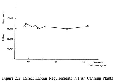
The paper on the fish canning industry by Cerbini and Zugarramurdi (1981a) shows manpower requirements lower than those given in Table 2.13; the reason is that the authors analysed plants where the heading and gutting process is mechanical and where cooking was done in a continuous cooker, whereas data in Table 2.13 refer to manual processing plants. Manpower requirements vary with the degree of mechanization and automatization of the plants. Other factors which have an influence on labour productivity and should be considered are: fish size, raw material quality, and workers' training level. In anchovy processing for fish salting poor raw material quality can decrease productivity up to 70%, and proper personnel training can increase productivity in 40 % (Montaner et al., 1994b). For instance Figure 2.6 shows the incidence of size and raw material quality in the production of cod fillets with skin.
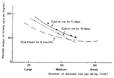
Figure 2.6 Production of Fillets with Skin as a Function of their Size and Quality
Table 2.14 and Figure 2.7 show how yield in the filleting operation varies according to the size of the fish and the experience of the operator (Amaria, 1974). Table 2.15 shows reduction in yield as a result of differences in fresh fish handling (Huss, 1988).
Table 2.14 Fillet Yield by Worker Experience and Size of Fish
Workers |
Experience (Years) |
Mean Size |
Mean Yield |
2 |
10 |
23.9 |
45.4 |
3 |
2 |
33.9 |
37.9 |
4 |
1 |
47.8 |
35.8 |
Table 2.15 Yield of Fillets made from Gutted Cod
Delay in Icing |
Fillet Yield (%) |
After Trimming |
1.0 h |
48.4 |
43.3 |
6.5 h |
46.5 |
40.4 |
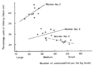
Figure 2.7 Fillet Yield by Size of Fish and Operator Experience
Figure 2.8 shows how the quantity of sardines to be headed and gutted by machine decreases as quality loss increases. However, productivity will be reduced also in manual plants since, to keep a given quality level, sardines have to be sorted by hand after visual inspection. From practical observations the sorting by hand of defective sardines, as is very often performed, is a cumbersome operation that requires a large surface (50-70 m2/t) and many workers. Quality continues to be lost during selection, and there is the possibility of a high increase in temperature in the fish handled, with an increased risk of histamine formation. Yield after the cooking operation also will be reduced, and a large number of broken sardines will appear in the cans as indication of bad quality. The same reasoning applies to the handling and processing of anchovies and other small pelagics. Quality loss in such cases could be assessed as the percentage of fish with belly-burst.

Figure 2.9 (Amaria, 1974) shows the estimated relationship between yield and filleting performance with and without incentives.
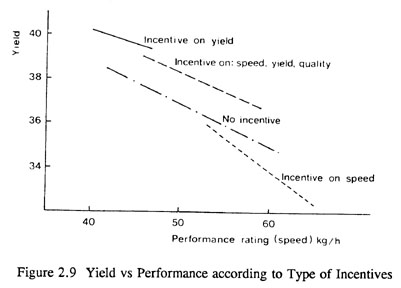
It can be concluded that an incentive on performance alone, results in a decrease in yield (from 38 to 34%). Incentives should therefore be given for a combination of performance, yield and quality (Kelsen et al., 1981).
Recent developments in work organization in the fishery industry tend to promote increase of performance, yield and quality through collective incentives (e.g., to the processing line) rather than individual incentives. This type of strategy, applied first in Scandinavian countries (not without initial difficulties) has proved to be successful both for workers and industry. Figure 2.10 shows the relationship between the size of the fish, the fillet yield and filleting performance, skinning and V-cut operation.
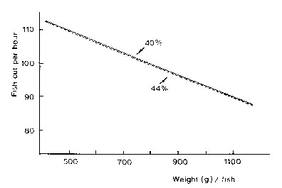
Figure 2.10 Number of Fish, Filleted, V-cut and Skinned vs Weight of Fish (g)
The graph shows that there is no correlation between yield and either the number of fish cut per hour or the size of the fish, which indicates that yield can be improved without affecting the quantity of fish cut per hour. As a result, there are no differences within the 40 to 44% yield range. It should be added that the greater the weight of the raw material, the smaller the quantity of fish that will be cut per hour. If the y-axis were expressed in terms of fish weight cut per hour, its relationship with the size of the fish would be positive, without affecting yield. Therefore it is more costly to use lighter weight fish for this line of production (Kelsen et al., 1981). In actual plants, hake less than 30 cm long is removed from the filleting line and processed as small H&G fish.
Example 2.13 Calculation of Direct Labour
Calculate the number of filleters required to produce 4 t of medium size cod fillet with skin, in a single shift of 8 hours, using cod which has been stored on ice for 5 days.
Answer: From Figure 2.6, for medium size cod fillets of 40 fillets/45 kg (40 fillets/ 100 lb), production rate will be around 250 fillets with skin/h.
40 fillets/45 kg corresponds to 1.125 kg/fillet
4 000 (kg/shift) / 1.125 (Kg/fillet) = 3 556 fillet/shift
3556 fillet/shift / ((250 fillet / (h x filleter)) x 8 (h/shift)) = 1.778 filleters, this means 2 filleters
The calculations made from Figure 2.6 pertain to the direct needs of the actual production activity (in this case, the filleting operation exclusively) and do not include the incidence of personnel necessary for moving raw material, finished products, and others. Those values will have to be added to the estimate already made.
Example 2.14 Labour Requirements for a Frozen Fish Plant
Calculate the quantity of labour needed for the frozen fish plant in Example 2. 1.
Answer: Worker production rate for each operation can be estimated from Table 2.13.
From Example 2.3 it is known that the plant will handle 5.9 t/day of raw material.
(i) Manual sorting workers (to clean, sort out, re-ice, and distribute fish).
According to Table 2.13, manual sorting can be done at a rate of 20-30 kg raw material/man x hour; the calculation is:
(5900 kg/shift) / (20 (kg/min) x 60 min/h x 8 h/shift) = 0. 61 man, say 1 worker
For a plant to start operation, it is convenient to utilize low production rates which should increase with time. From the calculation, one worker would appear to be enough. However, in practice this worker should also unload the trucks, wash the fish, re-ice the fish and clean fish boxes.
Manual cleaning of the fish boxes, corresponding to 5.9 t of raw material (about 200 boxes/day), will take no less than an additional five hours. This means that 2 workers will be needed at this stage.
(ii) Filleters (to fillet and skin the fish manually
According to Table 2.13, manual filleting and skinning of hake can be done at a rate of 40-52 kg (raw material)/man x hour; the calculation is:
5 900 kg/shift / [(40 kg / man x hour) x 8 hour/shift] = 18.43 men, say 19 filleters
To have an idea of the influence of productivity, the highest rate of production can be considered:
5 900 kg/shift / [(52 kg / man x hour) / 8 hour/shift] = 14.18 men, say 15 filleters
In this case, it is interesting to define a production policy. It is possible to start adopting the lowest production rate, the highest or one in between. In practice, it will depend on the skill of workers found on the work market, work laws, cost of manpower, possibilities to increase production (up to 2 additional tons of raw material, or about 34%), etc.
It should be noted that to take 19 filleters will require four additional positions in the filleting line (additional investment) and maybe additional facilities (e.g., bathrooms) and supervision. A possible compromise is to contract only 15 filleters and pay overtime initially.
(iii) Inspection and V-cut
To determine the number of inspectors (they could actually work as internal quality inspectors) the same considerations can be applied as for the previous point. From Example 2.4 it is known that 5.9 t of raw material produced 2.36 t of untrimmed fillets to go for trimming (inspection and V-cut):
2 360 kg/shift / ((67 kg / woman x hour) x 8 hour/shift) = 4.40 women, say 5 inspectors
Probably in this case, it would be advisable to contract five women so as to avoid risks regarding quality (note that in Argentina - from where the data were taken - women are assigned to this type of job because generally they are found to be more careful and tidy than men).
(iv) Packagers
Assuming that fillets will be packaged in blocks to be frozen, from Table 2.13 each packer (woman) will pack 81.8 kg per hour. The calculation is:
2 000 kg/shift / ((81.8 kg / woman x hour) x 8 hour/shift) = 3.05 women, say 3 packers
Please note that bag packaging, interleaved packaging or shatter packaging will give different results.
(v) General (or indirect) workers:
Table 2.13 gives the following figures:
10 filleters a general worker, this means 15 filleters 1.54 general workers, say 2 workers
5 packagers (or 5 inspectors) a general worker, this means 3 packers plus 4 inspectors (trimming and V cut) will require 2 workers.
In total 4 general (or indirect) workers.
(vi) Freezer attendant
According to Table 2.13, there is the need for one each 5 t of fish for freezing; in this case 2 t, which means that one cold storage attendant will be needed. This example makes it clear that a number of considerations should be made to produce actual calculations of manpower, even if reliable data are available.
The example makes it clear also how some aspects like quality, workers' skill and production policies can affect calculations. A "standard" plant does not exist, and noticeable differences can be found in practice even between similar plants of the same company, particularly when the degree of mechanization is low.
Example 2.15 Labour Requirements for a Fish Canning Plant
Calculate the labour requirements necessary for the canning plant in Example 2.2
Answer: From Table 2.13, average operation time is 2.5 min/can, which when calculated as hours/day is 0.042 h/can. Therefore 14 workers working 8 hours daily will be needed to complete production of 2 670 cans. This includes indirect labour.
Generally two values are required to calculate this component:
Specific consumption
Peak consumption
Figures for specific consumption are used as averages in the estimate and represent the average consumption of the service being considered, for a specific capacity of production.
Peak consumption is what can be produced in a case where the entire plant and all the equipment is operating at full capacity or when special equipment, which consumes more than average, is put into operation in the plant.
In fish processing industries, utilities (electricity, steam, water, natural gas and fuels) consumption varies over a wide range, depending on process technology and product characteristics. From the analysis of freezing, canning, cured fish and fishmeal plants, it was found that utilities consumption also depends on plant location (developed and developing countries), equipment characteristics (technology, maintenance and lifespan) and the source of the utilities (Montaner et al., 1994c). In Table 2.23 (at the end of the chapter) data on the consumption of these services are shown for different fish processing plants.
Electricity is used in two different ways:
for processes and lighting of the plant;
other uses: lighting the perimeters, administrative buildings, etc.
Consumption of electricity can be divided into two parts. At full production, a part (lighting, air conditioning of offices, etc.) approximately 20% of the total is practically constant and independent of production. The remaining 80% depends on production oil a non-linear basis. Energy consumption levels, as shown in Tables 2.16, 2.17 and 2.23, are also indicative and show variations which can be caused. For example, the consumption of electricity by the same type of freezer will obviously be greater in a tropical climate than in a temperate or cold one. This consumption can be reduced if walls and pipes are insulated, which will in turn increase fixed costs (set conditions exist for maximum thickness of insulation). Some equipment manufacturers produce "tropical" designs, which, besides being more insulated, have additional filters for air and fuel oil, more resistant materials at critical points and a higher or lower level of automation.
In practice, actual energy consumption, of any type, depends on the type of technology used and on the efficiency with which it is used. In developing countries, where the specialized labour for operation and maintenance is scarce or not properly trained, or where equipment must continue to be used well past its useful life because there is no capital for replacement, it is not difficult to find cases of energy consumption much higher than should be obtained from the initial characteristics and specifications of the equipment.
A typical case is that of ice production. In standard tropical conditions, the energy required to produce 1 t of ice varies between 50 and 90 kWh (see Table 2.23), where the lower value is for tube ice and the higher for flake ice. In a study carried out on four ice-making plants in Tanzania, the following values were found: 86, 117, 136 and 178 kWh, the lower value for block ice and the rest for flake ice plants. The energy requirements for the plants was therefore 40-110% higher than what could be expected. Problems, such as malfunction of pumps and fans, were identified in these plants (Anon., 1990).
The worldwide tendency it is to reduce and optimize the use of energy. Whereas in the past Governments were inclined to subsidize energy consumption to promote industry, in the future energy inefficient industries will be in practice penalized. This is not only due to the possible lack of oil, but also to the fact that reduction in oil consumption will reduce pollution. The fishery industry of developed countries, in particular those that lack oil (e.g., Iceland, Japan), have already started programmes to optimize energy consumption. Developing countries that should import oil (and use for that valuable hard currency) should become more concerned about energy consumption.
From the analysis of Table 2.23, it seems reasonable to extrapolate the consumption of electricity for canning plants to a value of 0.05 kWh/can of 170 g. Similarly, an average value of 200 kWh/t of finished product can be used for frozen fish plants and 140 kWh/t for fishmeal plants equipped with a unit to concentrate stickwater while for fishmeal plants without a concentration unit, this value decreases to 120 kWh/t of finished product.
In addition to the values of Table 2.23, Table 2.16 presents average values of energy consumption (electricity and fuels) in the New Zealand fishery and food industry.
Table 2.16 Energy Use in Fishery and Food Manufacturing Industry in New Zealand (1981) Data expressed as kWh of purchased energy per 1 kg of finished product (Cleland et al., 1981) (1)
Fuels |
Electricity |
||||
Product type |
Direct use in processing |
Allocated baseload |
Direct use in processing |
Allocated baseload |
Total |
Frozen whole fish and fillets |
0 |
0.222 |
0.175 |
0.722(2) |
1.111 |
Processed fish products (3) |
0.777 |
0.555 |
0.305 |
0.583 (2) |
2.222 |
Fishmeal |
3.361 |
0.333 |
0.361 |
0.055 |
4.111 |
Frozen poultry |
0.169 |
0.061 |
0.169 |
0.194 |
0.583 |
Frozen vegetables |
0.472 |
0.447 |
0.225 |
0.508 |
1.666 |
Processed meats (4) |
- |
0.972(2) |
- |
0.277(5) |
1.25 |
Notes:
Data do not include intra-factory transportation. No distinction is made between boiler fuel and fuel used in direct-fired equipment.
Includes energy used in refrigerated storage at the factory after processing but before distribution.
Average for canned fish, smoked fish fillets and battered, reformed fishery products.
Data represent the majority of the industry but are not representative of the industry as a whole.
Insufficient data existed to divide into direct use in processing and allotted baseload.
If available, natural gas can be utilized instead of fuel oil. At the same time, according to the technology utilized and the cost of the different sources of energy, the proportion between the different types can vary. In Table 2.17, data on energy consumption (electricity plus gas) of an American fish processing company are presented.
Table 2.17 Annual Energy Consumption (gas and electricity) 1981-83 Production Rate and Energy Consumption per 1 kg of Finished Product for a Fresh and Frozen Fish Processing Plant in the USA (adapted from Enriquez et al., 1986)
Element |
1981 |
1982 |
1983 |
Natural gas use (1) |
164237.6 (21.6%)(4) |
150580.4 (21.7%)(4) |
168 838.8 (20.1%)(4) |
Electrical energy use (1) |
608 124.4 (78.4%)(4) |
540 923 (78.3%)(4) |
670 285 (79.9%)(4) |
Total energy use (1) |
772 362 |
691 503.4 |
839 123.8 |
Total product output (2) |
567806.9 |
632 652.3 |
702 024.9 |
Energy consumption per 1 kg of final product (3) |
1.360 |
1.093 |
1.195 |
Notes: (1) in kWh; (2) in kg; (3) kWh/kg (final product); (4) % of total energy consumption
It is also necessary to know the fuels and steam consumption of the process. This is usually given by the equipment manufacturers. However, consumption may be different in practice. Steam consumption can basically be divided into three groups:
Steam for processes
Steam for electricity generation
Steam for other uses (heating, laboratories, cleaning)
Tables 2.16 and 2.23 show the consumption of fuels in general and fuel oil necessary to supply steam to processing plants. The ratio used in technical estimates is between 14 and 22 kg of steam/kg of fuel oil (Lisac, 1974; Vaaland and Piyarat, 1982).
For fish canning plants, the maximum value can be estimated at 0.05 kg fuel oil/170 g can, although it should be pointed out that the figure resulting from calculating only the thermal treatment parameters can cut this value by half. For fishmeal plants, a consumption of 140 to 190 kg fuel-oil per ton of finished product can be estimated, depending on the existence or not of a concentration unit.
Water can be used for different purposes in a plant. The following uses could be considered:
Processing water
Refrigeration water
Boiler water
Water for general and human use
Each type of water may require special treatment. Sources of water for a factory are usually:
Well water
Surface water (river, lake, etc.) or sea water
Tap water
In the fish processing industry, operations can vary from one plant to another, but the quantity and quality of water used in a similar process are the same and depend directly on the capacity of the plant. Current tendency is towards design of fish washing machines functioning with reduced amounts of water; this is part of the "clean production" approach. By achieving appropriate washing with less water, the overall water requirement is reduced and so is the amount of liquid wastes (reduction in the installed capacity and cost of liquid waste treatment). Table 2.18 lists percentage of water requirements for the production of frozen white fish fillets.
Table 2.18 Percentage of Water Used in Different Operations in the Production of Frozen White Fish Fillets in Canada (Blackwood, 1978)
Operation |
Total water consumption (%) |
Water transport of fish fillets and waste |
50-65 |
Cleaning, scaling of fish, preparation of fillets, and skinning |
15 -25 |
Cleaning of plant, boat, wharf, etc. |
12- 18 |
Manufacture of fishmeal |
2- 4 |
Manufacture of ice |
1 - 3 |
Fresh water for fishing boats |
1 - 2 |
Baths and sinks |
1 - 2 |
Water for boilers, refrigeration, etc. |
1 - 2 |
Manual fish washing is done usually in large bats (made out of concrete, stainless steel or plastic); shallow baths (about 0.5 m deep) allow better washing. Washing procedure can be batch type for both water and fish or batch-wise for fish and with a water overflow. Water requirements are in the order of 03-1 m% of fish to be washed. As water requirements for washing are proportional to the surface to wash, small pelagics will require more water than medium size and large fish per ton of fish to be washed.
Plenty of water is required in fish and fish fillet washing. Table 2.18 shows water consumption for seven different fish washing machines. Table 2.19 also shows the influence of different types of technological alternatives on water consumption during fish washing.
Table 2.19 Water Consumption in Fish and Fish Fillet Washing Machines
Type of machine |
Machine capacity (t/h) |
Water consumption |
Consumption per ton of fish (m3/t fish) |
Reference |
Herring washer (1) |
2 |
4/6 m3/h |
2-3 |
Baader 654 (7) |
Raw fish washer (2) |
5-6 |
15/20 " |
2.5-4 |
Baader 670 (7) |
Fish washer (3) |
3 |
0.6 m3 (5) |
- |
Baader 679 (7) |
| Washing, de-bleeding and brining drum (3) | 2 |
0. 3 m3 (5) |
- |
Baader 676 (7) |
Standard drum washer (4) |
- |
- |
1 |
Blackwood (1978) |
Washing bat |
0.53.5(6) |
0.6 m3/h |
1.2-0.17 (6) |
Model MK5 (8) |
Washing bat |
1.5-10(6) |
0.6 m3/h |
0.4-0.06 (6) |
Model MK 8 (8) |
Notes:
Batch washer
Continuous washer
Continuous washer, however, part of water is retained (overflow)
Standard drum washer (see design in Blackwood, 1978)
This is only the initial charge of tub, overflow should be added
Capacity depends on fish residence time in the washer (adjustable from 3 to 20 min)
Data taken or calculated from Baader catalogue (English version) for 1988
Data taken or calculated from K.M. Fish Machinery A/S (DK) Catalogue for 1994
Fish processing also requires large amounts of water. Table 2.19 presents data on water requirements for some machine fish-processing operations. A completely mechanized white fish fillet processing line will require, according to Tables 2.19 and 2.20, 4.5-6 m3, of processing water per ton of fillets produced. Actual water consumption should be calculated according to machine specifications, characteristics of fish to process and worker skills.
Fish, fillets and shrimps can be transported within a processing line by conveyors (dry method) or by a flow of water (wet method). The wet method requires very large amounts of water as can be seen from Table 2.23 (Blackwood, 1978). The amount of water required for hydraulic conveyors depends on the fish size; small sized fish require 3-4 m3/t, medium sized fish 4-6 m3/t and large sized fish 6-8 m3/t (Chupakhin and Dormenko, 1965).
Not all water has to be drinking water; much of it, depends on its use (e.g., fish washing and hydraulic transport) can be, clean seawater. Of the very large values reported by Blackwood (1978) on water consumption in the Canadian fishery industry (see Table 2.18) most of them (between 98.5 and 95%) correspond to clean seawater. However, today, the tendency is to reduce this large amount of clean seawater because it can easily become a source of pollution (harbours, bays and rivers) and increase waste treatment costs.
Table 2.20 Water Requirements of Some Fish Processing Machines
Type of machine |
Machine capacity (No. of fish/min) (1) |
Machine capacity (t/h) |
Water consumption (m3/t) (1) |
Water consumption per t processed (m3/t) |
References |
Grading (shrimp) |
- |
0.5 (1) |
1.5 |
3 |
Model KM500 (5) |
Grading (shrimp) |
- |
1 (1) |
1.5 |
1.5 |
Model KM1000 (5) |
Grading (small pelagics) |
- |
15 (herring) (1) |
2.1 |
0.14 |
Model KM231 (5) |
Grading (white fish) |
- |
up to 18 (1) |
1.2 |
0.06 |
Baader 486 (6) |
Gutting (white fish) |
25-40 |
3.5 (2) |
1.5 |
0.43 |
Baader 160, 161, 162 (6) |
Gutting (white fish) |
40-60 |
5(2) |
1.8 |
0.36 |
Mark 5 (5) |
Nobbing (small pelagics) |
460 |
0.6 (2) |
0.9 |
1.5 |
Baader 464 (6) |
Filleting |
24-34 |
1.5 (2) (3) |
0.9 |
0.6 |
Baader 189 (6) |
Filleting |
40-65 |
1.8 (2) (3) (4) |
2.4 |
1.33 |
Baader 190(6) |
Skinning |
30/140 |
1 (2) (3) |
0.09 |
0.09 |
Baader 51 (6) |
Notes:
According to manufacturers data
Calculated from manufacturers data and average data on processed fish species. Capacity can change according to actual fish size and operator skill
Result expressed in t/h of fillets produced
In this case, the machine produces V cut fillets
Data taken from K.M. Fish Machinery A/S (DK), catalogue for 1994
Data taken from Baader catalogue (English version) for 1988
Example 2.16 Services Requirements for a Frozen Fish Plant
Estimate consumption of water and energy for the frozen fish plant in Example 2. 1.
Answer: Values can be estimated from Tables 2.16 and 2.23.
Energy consumption. Total energy consumption can be estimated as 1. 111 kWh/kg finished product (see Tables 2.16 and 2.17); i.e., for 2 t of final product, the total energy required for processing and refrigerated storage before distribution will be 2 222 kWh. Of this total, around 80% (Tables 2.16 and 2.17), 1776 kWh, will correspond to electricity and the remaining 20% (444 kWh) should be provided by fuels (fuel oil or gas or a mixture of both). The energy consumption directly related to production can be calculated in order to obtain the component of the production cost. From Table 2.23 the average value is 200 kWh/t of finished product; therefore 400 kWh will be required daily to produce 2 t of fillets.
Water consumption. In this case, gutting, filleting and skinning will be done by hand; from the data provided by Zugarramurdi (1981a) (see Table 2.23), 4 m3 for direct fish processing will be enough. Assuming fish is washed in a standard drum washer, 5.9 m3 should be added for 5.9 t of raw material, which means a total of 9.9 m3 for fish processing only. Taking into account Table 2.18 and that, in this case, it is dry processing, the rest of water (cleaning of plant and boxes, baths and sinks and water for boiler and refrigeration) will be around 47-49 % of total water requirements; this means an additional 9.14 m. In total (9.9 m3 + 9.14 m3) 19.04 m3 of water are required for 2 t of fillets. The lowest figure of Blackwood (1978) data (see Table 2.23) would be 28 m3, which is a much higher value (47 % above). In this case, the estimate of 19 m3 seems acceptable. This example clarifies the need to determine directly whenever possible, water consumption. As observed by Blackwood (1978) wide differences are found in water consumption and it is an indication of water wastage.
Example 2.17 Services Requirements for a Fish Canning Plant
Calculate the consumption of water, electricity and fuel for the canning plant in Example 2.2. Daily production is 2 670 cans of tuna of 180 g each.
Answer: According to initial data, the plant will produce 2 670 tuna cans per day of 180 g each, i.e, daily production will be 0.4806 t (in this case, fish and oil together are considered product). Table 2.21 can be constructed from data in Tables 2.16 and 2.23:
Table 2.21 Energy and Water Consumption in a Fish Canning Plant
Reference |
Electricity |
Fuels |
Total Energy |
Water |
Table 2.23 (1) |
122 kWh/day |
1643 kWh/day (4) |
1 787 kWh/day |
34 m3 /day |
Table 2.23 (2) |
21 kWh/day |
552 kWh/day (4) |
573 kWh/day |
13.5 m3/day |
Table 2.16 (3) |
641 kWh/day |
427 kWh/day |
1 068 kWh/day |
- |
Notes:
Data from Myrseth (1985) on tuna canning (automatic processing line).
Data from Edwards (1981) on sardine canning in tropical countries (manual processing).
Data from Cleland et al. (1981) processed fishery products in general (including energy used in refrigerated storage).
Conversion factor: 11.955 kWh per 1 kg of fuel oil.
Table 2.21 allows us to make the following analysis:
Total energy consumption will be in the order of 573-1787 kWh/day, and 0.218-0.67 kWh/can.
Water consumption will be in the order of 5-12.7 1/can.
Fuel oil consumption will, in this case, be more important than electricity consumption, between 92 and 96% of the total.
Edwards' (1981) data differ from Myrseth' s (1985) data by 68% regarding total energy consumption and 60% regarding water consumption. The large difference in values could be due to the large degree in mechanization and automation in the Norwegian plant considered by Myrseth (1985).
In conclusion, an average of the data of Edwards (1981) and Myrseth (1985) can be adopted as the best estimate in this case. This example also shows that any application of data from Table 2.23 (or in any other table) should be carefully analysed during calculations and cross references checked whenever possible.
Packaging is usually considered within the raw material inputs. However, it was decided to discuss it separately because in some cases in the fishery industry it can represent a large percentage of total production costs. Table 2.22 shows the consumption of packaging materials for different products.
Table 2.22 Packaging Requirements in the Fishery Industry
Type of Packaging |
Packaging Requirements |
References |
Frozen* |
||
Interleaved fillets |
15 kg polyethylene/t product |
|
Waxed cartons, 7 kg each |
150 boxes/t product |
|
Master cardboard boxes, 21 kg each |
50 boxes/t product |
|
Straps |
1 kg/t product |
|
Labels |
50 labels/t product |
|
Canned* |
||
Thermoplastic Packaging |
36 cans x 115 g |
|
36 cans x 170 g |
||
24 cans x 260 g |
||
Corrugated cardboard box |
1 box/24 cans x 380 g |
|
Fishmeal |
||
Bags (50 kg/bag) |
22 bags/t fishmeal |
(Shaw, 1976) |
Salted |
||
Drums x 50 1 |
17.6/t fresh fish |
(Perovic, 1990) |
Smoked (240 fish at 500-600 g ea.) |
||
Trays |
120 |
(FAO, 1986a) |
Self-sticking tape |
48 m |
" |
Labels |
120 |
" |
*Standard consumption in Argentina
Example 2.18 Packaging. Requirements for a Frozen Fish Plant
Calculate the packaging requirements for the daily production of the frozen fish plant in Example 2. 1. Daily production is 2 t of frozen fish blocks.
Answer: Daily consumption of packaging can be calculated from the values of Table 2.22.
300 waxed cartons
100 master cardboard boxes
2 kg straps
100 labels
Example 2.19 Packaging Requirements for a Fish Canning Plant
Calculate the packaging requirements for the canning plant in Example 2.2.
Answer: The following values are obtained from the data given in Tables 2.2 and 2.22
2 670 cans of 180 g each
115 corrugated cardboard boxes x 24 cans
In this section, several references illustrate the relationship between yield, inputs and quality. Today, it is felt that the task of quality assurance also includes analysis and control of yield and inputs for a plant (Huss, 1992). This concept, which in practice is significantly different from the classic concepts of fish inspection and quality control, is justified by the fact that quality assurance requires a more detailed, rational and dynamic knowledge of the processes. This in turn involves the analysis and control of yield, inputs, work conditions and safety (which influences the work force) and reduction of losses and/or all types of waste. This information is in turn linked to costs, to be analysed in Chapter 4.
Table 2.23 Manpower and Services Consumption for Fish Plants
Type of Plant/Capacity (t of RM/time) |
Direct Manpower (No. workersh FP) |
S,A (1) |
Water (m3/t FP) |
Electricity (kWh/t FP) |
Fuel-oil (kg/t FP) |
Data calculated from |
Canning Plant |
||||||
21day (Manual H&G) |
112 |
n/a |
375/day |
n/a |
n/a |
Shaw, 1976 (Tropical Countries) |
2/day (Mechanical H&G) |
62 |
- |
- |
- |
- |
" |
20-30/day (Mechanical H&G) |
30 |
S: 1/20 |
n/a |
n/a |
n/a |
" |
Sardines n/a |
- |
- |
- |
25 |
90 |
Lisac, 1974 |
| Sardines: 2/day (Mechanical H&G) | 82.5 |
S: 1/33; A: 1/22 |
28 |
59 |
96 |
Edwards el al., 1981 (Tropical Countries) |
Sardines: 2/day (Manual H&G) |
140 |
S: 1/56; A: 1/37 |
28 |
44 |
96 |
" |
| Sardines: 17/day (Mechanical H&G) | 31 |
S: 1/20 |
n/a |
294 |
294 |
Zugarramurdi, 1981b (Argentina) |
Sardines: 15/8 h (Mechanical H&G & Packaging) |
8 |
S: 1/15; A: 1/5 |
57 |
226 |
174 |
Myrseth, 1985 (Norway) |
Smoked Sardines: 5/8 h |
20 |
S: 1/13; A: 1/6 |
74 |
308 |
147 |
" |
| Tuna: 20/8 h (Automatic production line) | 9 |
S: 1/18; A: 1/8 |
71 |
300 |
286 |
" |
SkipJack: 10/8 h |
9 |
S: 1/9; A: 1/7 |
62 |
489 |
221 |
" |
Salmon: 8/8 h |
n/a |
n/a |
52 |
196 |
204 |
" |
Shrimp: 3.6/8 h |
n/a |
n/a |
206(2) |
580 |
237 |
" |
Fish Freezing Plants |
||||||
2/day |
25-31 |
n/a |
36 |
n/a |
n/a |
Shaw, 1976 (Tropical Countries) |
20/day |
10-12 |
n/a |
n/a |
n/a |
n/a |
" |
Shrimp: 4/8 h.processing |
5 |
S: 1/10 |
240 |
200 |
n/a |
Bartholomai, 1987 (USA) |
Shrimp: 1.6/day |
51 |
S: 1/8 |
1.3 |
1 111 |
n/a |
Street et al., 1986 (Tropical) Countries) |
Whole fish 4.48 t FP/8 h |
4 |
S: 1/6 |
1.2 |
446 |
n/a |
" |
Catfish: 26/8 h (6) |
2 |
S: 1/28 |
14.4 |
105(7) |
n/a |
Bartholomai, 1987 (USA) |
Hake fillet: 25/day |
9 (13) |
S: 1/20 |
2(12) |
588 |
n/a |
Zugarramurdi, 1981a (Argentina) |
Whole and filleted fish |
n/a |
n/a |
n/a |
897 |
n/a |
Cleland et al., 1981 (New Zealand) |
Croaker (H&G) |
7 |
n/a |
n/a |
n/a |
n/a |
Kelsen et al., 1981 (Uruguay) |
Whole croaker |
3 |
n/a |
n/a |
n/a |
n/a |
" |
Hake and whiting fillets |
11-13 |
n/a |
n/a |
n/a |
n/a |
" |
White fish fillets (dry transport) |
n/a |
n/a |
14-32 |
n/a |
n/a |
Blackwood, 1978 (Canada) |
White fish fillets (wet transport) |
n/a |
n/a |
83-275 (2) |
n/a |
n/a |
" |
Cold Storage |
||||||
10 t fresh fish/24 h |
n/a |
n/a |
n/a |
0.5 |
n/a |
Lisac, 1974 |
10 t frozen fish/24 h |
n/a |
n/a |
n/a |
1 |
n/a |
" |
Ice Production |
||||||
Ice |
n/a |
n/a |
n/a |
50-90 |
n/a |
Lisac, 1974 |
Tubelflake ice (Temperate Zone) |
n/a |
n/a |
n/a |
45-60 |
n/a |
Myers, 1984 |
Tube/flake ice (Tropical Zone) |
n/a |
n/a |
n/a |
60-85 |
n/a |
" |
Fishmeal Plants |
||||||
n/a |
n/a |
n/a |
n/a |
175 |
200 kg |
Lisac, 1974 |
20/8 h |
1 |
n/a |
n/a |
n/a |
n/a |
Shaw, 1976 (Tropical Countries) |
200/8 h |
0.3 |
n/a |
n/a |
n/a |
n/a |
" |
10-60124 h (8) |
1 |
n/a |
90 |
120 |
140 |
FAO, 1986c |
100-200/24 h (8) |
0.6 |
S: 1/7 |
62 |
112 |
136 |
" |
250-500124 h (8) |
0.3 |
S: 1/8 |
50 |
104 |
132 |
" |
10-60124 h (9) |
n/a |
n/a |
126 |
140 |
220 |
" |
100-200124 h (9) |
n/a |
n/a |
90 |
132 |
192 |
" |
250-500124 h (9) |
n/a |
n/a |
73 |
124 |
180 |
" |
Salted |
||||||
Anchovy: 1 000/day |
23(10) |
n/a |
14 |
35 |
n/a |
Perovic, 1990 (Mexico) |
Dried |
||||||
Mechanical: 0.654112 h |
23 |
n/a |
n/a |
170 |
395 (11) |
Waterman, 1977 (African Countries) |
Manual: 0.654112 h |
47 |
n/a |
n/a |
n/a |
n/a |
" |
Protein Concentrate |
||||||
FPC, type A: 200/day |
0.15 |
n/a |
49 |
230 |
53 |
Almenas et aL, 1972 |
| FPC, type B: 56-8/day | 1.8 |
n/a |
n/a |
223 |
223 |
Vaaland & Piyarat, 1982 (Brazil) |
Silage: 6 t FP/day |
0.33 |
n/a |
n/a |
n/a |
n/a |
Bertullo, 1989 (Uruguay) |
Smoked |
||||||
Small Fish (driedlsmoked) 4.3/day |
13 |
1/6 |
n/a |
2.6 m wood |
n/a |
Waterman, 1977 (Tropical Countries) |
Marine Beef |
||||||
Mechanical Processing: 120/day |
3 |
n/a |
15.9 |
2.493/t FP |
n/a |
Vaaland & Piyarat, 1982 (Brazil) |
Marinated |
||||||
Herring |
n/a |
n/a |
21 |
n/a |
n/a |
Blackwood, 1978 (Canada) |
RM: Raw Material
DM: Direct Manpower
FP: Finished Product
H&G: Headed and Gutted
Notes:
S: No. of Supervisors/No. of Workers; A: No. of Administrative/No. of Workers
The raw material is transported by flowing water and gravity
Assuming a raw material yield of 40%
Manual packaging (rest mechanized), with shrimp being moved by water
With ice plant, RM and FP cold storage
Three types of product are made: H&G, fillets and fish balls
Note, the refrigeration equipment consumes 1.3 t CO2/t FP
With indirect steam drier, without evaporation plant. Compact line
With indirect steam drier, with evaporation plant
Final salted product: 915 t
Diesel Oil
Only fish processing consumption (it does not include washing)
Overtime was part of the production scheme
![]()
![]()
![]()