1 With contributions from J. L. Teixeira, Instituto Superior de Agronomia, Lisbon, Portugal.
COMPLETING A DATA SET
Quite often data sets containing a weather variable Yi observed at a given station are incomplete due to short interruptions in observations. Interruptions can be due to a large number of causes, the most frequent being the breakage or malfunction of instruments during a certain time period. When data are missing, it may be appropriate to complete these data sets from observations Xi from another nearby and reliable station. However, to use portions of data set Xi to replace data set Yi, both data sets Xi and Yi must be homogeneous. In other words, they need to represent the same conditions. The procedure for completing data sets is applied after the test for homogeneity and any needed correction for nonhomogeneity has been performed. The substitution procedure proposed herein consists of using an appropriate regression analysis.
The procedure for substituting nearby data into an incomplete data set can be summarized as follows:
1. Select a nearby weather station for which the data set length covers all periods for which data are missing.
2. Characterize the data sets from the nearby station, Xi, and of the station having missing data, Yi, by computing the mean  and the standard deviation sx for the data set Xi:
(4-1)
(4-2)
and the mean  and standard deviation sy for data set Yi:
(4-3)
(4-4)
for the periods when the data in both data sets are present, where xi and yi are individual observations from data sets Xi and Yi, and n is the number of observations in each set.
3. Perform a regression of y on x for the periods when the data in both data sets are present:
(4-5)
with
(4-6)
(4-7)
where a and b are empirical regression constants, and covxy is the covariance between Xi and Yi. Plot all points xi and yi and the regression line for the range of observed values. If deviations from the regression line increase as y increases then substitution is not recommended because this indicates that the two sites have a different behaviour relative to the particular weather variable, and they may not be homogeneous. Another nearby station should be selected.
4. Compute the correlation coefficient r:
(4-8)
Both a high r2 (r2 ³ 0.7) and a value for b that is within the range (0.7 £ b £ 1.3) indicate good conditions and perhaps sufficient homogeneity for replacing missing data in the incomplete data series. These parameters r2 and b can be used as criteria for selecting the best nearby station.
5. Compute the data for the missing periods k = n+1, n+2..., m using the regression equation caracterized by the parameters a and b (equations 4-6 and 4-7), thus
(4-9)
6. The complete data set with dimension m will now be
Yj = yi (j = i = 1,...,n) (4-10)
(j = k = n + 1, n + 2,...,m)
Note that estimates  taken
from the regression equations are useful for predicting evapotranspiration.
However, they cannot be treated as random variables (2).
2 To create random values,, one can add to(equation 4-9) the residuals e k synthetically generated from a population N (0, sy, x). The residuals are created using tables of random numbers. In that case the estimates Yj can be treated as random variables.
ANALYSIS OF THE HOMOGENEITY OF DATA SERIES
Weather data collected at a given weather station during a period of several years may be not homogeneous, i.e., the data set representing a particular weather variable may present a sudden change in its mean and variance in relation to the original values. This phenomenon may occur due to several causes, some of which are related to changes in instrumentation and observation practices, and others which relate to modification of the environmental conditions of the site, such as rapid urbanization or, on the contrary, perhaps development of irrigation in the area.
Changes relative to data collection may be caused by:
· change in type of sensor or instrument;· change in the observer and or change in the timing of observations;
· "sleeping" data collector;
· deterioration of sensors, such as with some types of pyranometers and RH sensors, or malfunctionning of mechanical parts, such as with a tipping bucket rain gauge, or by an intermittently broken or snorted wire;
· aging of bearings on anemometers;
· use of incorrect calibration coefficients;
· variation in power supply or electronic behaviour of instruments;
· growth of trees or planting of tall crops or construction of buildings or fences near a raingauge, anemometer, or evaporation pan;
· change in the location of the weather station, or in the types of shelters for housing temperature and humidity sensors;
· change in the watering, type or maintenance of vegetation in the vicinity of the weather station;
· significant change in the watering or type of vegetation of the region surrounding the weather station.
These changes cause observations made prior to the change to belong to a statistically different population than data collected after the change. It is therefore necessary to apply appropriate techniques to evaluate whether a given data set can be considered to be homogeneous and, if not, to introduce the appropriate corrections. To do so requires the identification of which sub-data series is to be corrected. To do this requires local information.
Procedures indicated herein are simple but are well proven in practice. They rely upon the statistical comparison of two data sets, one considered homogeneous and constituted by the observations Xi, the other being the one under analysis and constituted by the observations Yi of the same weather variable (Tmax, Tmin, u2, RHmax,..., etc). Both sets Xi and Yi should be collected at two stations that are in the same climatic region, i.e., Xi and Yi should present the same trends in time despite the space variability when short time scales (daily, weekly or decadaily) are utilized.
The reference observations Xi are selected from a weather station for which the data set can be considered to be homogeneous. (3) The Xi data set should have the same time length of observations as the set of observations Yi.
3 When, for a given climatic region, there is no information concerning the homogeneity of data, then the average of observations of the same variable from all stations (excluding the one in the analysis),, can be used to constitute the homogeneous data set.
Method of Cumulative Residuals
When relating two weather data sets from two weather stations, where the first is considered to be homogeneous, the data set of the second station can be considered to be homogeneous if the cumulative residuals of the second data set from a regression line based on the first data set are not biased. The bias hypothesis can be tested for a given probability p. This is done by verifying whether the residuals can be contained within an elipsis that has axis a and axis b. The magnitudes of a and b depend on the size of the data set, on the standard deviation of the sample being tested and on the probability p used to test the hypothesis (4).
4 This test utilizes results from residuals from the linear regression of Y on X. The residuals should follow a normal distribution with mean zero and standard deviation sy, x, i.e. the error e i Î N (0, sy, x). The residuals from the regression should be considered to be independent random variables (i.e., they should exhibit homoscedaticity).
The procedure for analysing the homogeneity of a weather data set Yi collected in a given weather station environment can be summarized as follows:
1. Select a reference weather station inside the same climatic region that is known to have an homogeneous data set Xi of the same weather variable. As an alternative, construct a "regional" homogeneous data set by averaging the observations at several weather stations in the same region.
2. Organize both data sets xi and yi in chronological order i = 1, 2,..., n, where the starting time and time increment are identical for both data sets.
3. For both data sets, compute the mean and standard deviation (equations 1 to 4) for the homogeneous variable (xi) and for the variable to be tested (yi).
FIGURE 4.1. Regression between two sets of weather data, with the X data set being homogeneous. The example shows that the homoscedescity condition was satisfied.
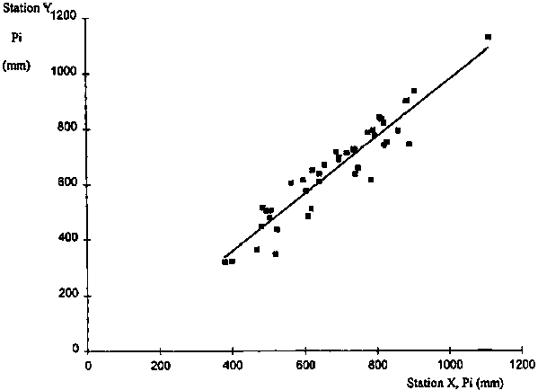
4. Calculate the regression line between the two variables yi and xi and the associated correlation coefficient (equations 4-5 to 4-8). The regression equation among the full sets is expressed as
(4-11)
where the subscript f refers to the full set. Whenever possible, plot xi, yi and the regression line to visually verify whether the homoscedaticity hypothesis (5) can be accepted (see Figure 4.1)6
5 The homoscedaticity hyphotesis is accepted when the residuals e i of the dependent variable to the regression line (equation 4-5) can be considered to be independent random variables. This can be visually assessed when the deviations of yi to die regression estimatesare within the same range for all xi, i.e., when these deviations are not increasing (or decreasing) with increasing values of xi.
6 Data in this example were provided by J. L. Teixeira (personal communication, 1995).
5. Compute the residuals of the observed yi values to the regression line (equation 4-5), the standard deviation sy, x of the residuals and the corresponding cumulative residual Ei:
(4-12)
(4-13)
(4-14)
6. Select a probability p for accepting the hypothesis of homogeneity. The value p = 80% is commonly utilized. Then compute the elipsis equation having axes
a = n/2 (4-15)
(4-16)
where:
n size of the sample under analysis
zp standard normal variate for the probability p (usually p = 80% for non excedancy): Table 4.1
sy, x standard deviation of the residuals of y (equation 4-13)
The parametric equation of the elipsis is then
X = a cos (q) (4-17)
Y = b sin (q)
with q [rad] varying from 0 to 2 p.
TABLE 4.1. Value of the standard normal variate zp for selected probabilities P of non-excedance
|
p (%) |
zp |
p (%) |
zp |
|
50 |
0.00 |
80 |
0.84 |
|
60 |
0.25 |
85 |
1.04 |
|
70 |
0.52 |
90 |
1.28 |
|
75 |
0.67 |
95 |
1.64 |
Note: given the symmetry of the normal distribution, the values for p < 50% correspond to (100 - p) but with the opposite sign. Ex: p = 20% is associated with z = -z80 = -0.84
It can therefore be concluded, at the level of probability p, that there is no bias in the distribution of residuals, i.e., the data set yi is considered to be homogeneous, when the computed values for Ei fall inside the elipsis (equation 4-17).
7. Plot the cumulative residuals Ei against time using the time scale (interval) of the variable under analysis (Figure 4-2).
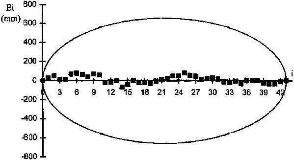
8. Draw the elipsis on the same plot and verify whether the Ei all lie inside the elipsis. If they do, then the hypothesis of homogeneity is accepted at the p level of confidence (Figure 4.4).
FIGURE 4.2. Plot of cumulative residuals against time and associated elipsis for the probability p = 80%, with results indicating that data set Y is not homogeneous (relative to data set X).
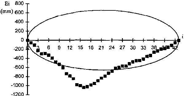
9. If the hypothesis of homogeneity cannot be accepted (this is the case in Figure 4.2), then one can select the break point where it appears that Ei ceases to increase (or to decrease) and begins to decrease (or to increase), for example at I = 16 in Figure 4.2. This break point is termed k = i.
10. The data set is now divided into two subsets, the first from 1 to k, the second from k + 1 to n. Then, new regression equations are computed between Y and X for both subsets. If we presume that the second subset is homogeneous but that the first is not, then we have
(4-18)
and
(4-19)
where the subscripts h and nh identify the regression coefficients of the homogeneous and the non homogeneous subsets, respectively (see Figure 4-3).
11. Compute the differences between the two regression lines
(4-20)
for the non homogeneous set (i = 1, 2,...,k)
FIGURE 4.3. The regression lines for the two subsets obtained from the data sets of Figures 4.1 and 4.2. Selection was made after definition of the break point in Figure 4.2.
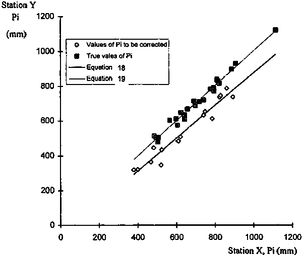
FIGURE 4.4. Plot of cumulative residuals against time and the associated elipsis for p = 80% after correction of variable y.
12. Correct the non homogeneous subset portion of data set
(4-21)
where the subscript c identifies the corrected values. Thus, the corrected, homogeneous full set for weather variable Y is composed by
Yi = yc, i for i = 1, 2,..., k (4-22)Yi = yi for i = k + 1, k + 2,..., n
A similar procedure would be utilized if it was presumed that the second sub-set requires correction, rather than the first sub-set.
Note that the variables Yi are still considered to be random variables despite that the mean and the variance have been modified due to the correction introduced. To confirm the results of the correction of data set Y for homogeneity, the homogeneity test methodology can be applied again to the corrected variable Y to provide evidence of homogeneity in the graph of residuals. This has been done in Figure 4.4.
In this example, it was presumed that the latter sub-set (k to I) was the correct (representative) data set, or the data set displaying the desired attributes. It was therefore presumed that prior to time k, the readings were biased by instrument calibration, different location of the station or the instrument within the station, change in type or manufacturer of the instrument, or change in general environment of the station. It appears in Figure 3 that the data prior to i = k were biased downward by approximately 100 mm of annual precipitation.
Double-Mass Technique
The double-mass technique is also useful for assessing homogeneity in a weather parameter. As with the method of cumulative residuals discussed in the last section, the double-mass technique requires data sets from two weather stations, where Xi (i = 1, 2,..., n) is a chronologic data set for a given weather variable observed for a certain time length at a "reference" station, and which is considered to be homogeneous, and where Yi is a data set of the same variable, with the same time length, observed at another station and for which homogeneity needs to be analysed.
In the double-mass technique, starting with the first observed pair of values X1 and Y1, cumulative data sets are created by progressively summing values of Xi and Yi to verify whether the long term trends in variation of Xi and Yi are the same. Thus the following cumulative variables are obtained
(4-23)
and
(4-24)
with i = 1,..., n and j = 1,..., i - 1.
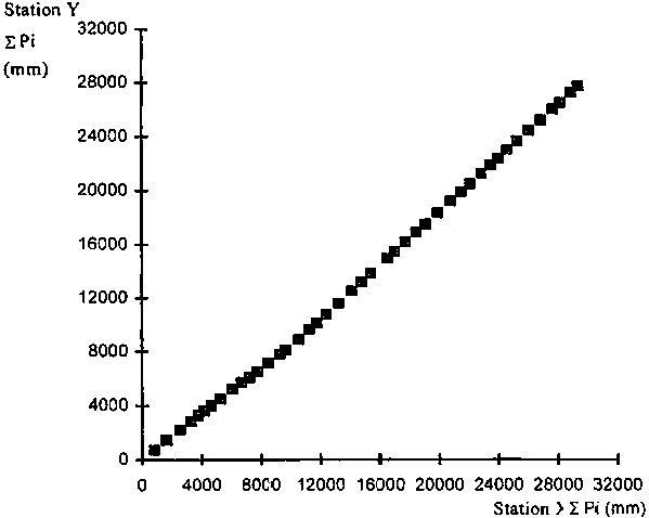
FIGURE 4.5. Double mass analysis applied to two series of precipitation when data from station Y are not homogeneous
These variables xi and yi are still considered to be random variables and are characterized by the mean and the standard deviation (equations 4-1 to 4-4). The yi and xi variables can be related through linear regression (equations 4-5 to 4-8). However, the double mass technique is typically applied as a graphical procedure.
The graphical application of the double-mass analysis is done by plotting all coordinate points xi and yi. The plot is then visually analysed to determine whether successive points of xi and yi follow an unique straight line, indicating the homogeneity of the data set Yi relative to data set Xi. If there appears to be a break (or more than one break) in the the plot of yi to xi, then there is a visual indication that the data series Yi (or perhaps Xi) is not homogeneous (Figure 4.5). The break at coordinates xk and yk can be used to separate two subsets (i = 1, 2,..., k) and (k + 1, k + 2,..., n). One of the subsets is to be corrected. The appropriate one to correct needs to be identified by consulting the records of the weather station, when available.
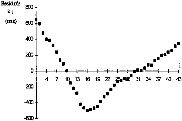
FIGURE 4.6. Residuals of double mass to the straight line (equation 26) indicating the non homogeneity of the residuals of the series of precipitation of station Y.
Often, visual interpretation of the double-mass balance is difficult. Thus the following numerical regression procedure is recommended:
1. Compute the regression line through the origin for the full set of data xi and yi
(4-25)

2 Compute the residuals to the regression line
e i = yi - b xi (4-26)
3. Analyse the distribution of residuals. If the residuals plot as independent, random variables, then the set can be considered to be homogeneous. However, if the distribution of residuals is biased over i = k, then the. homogeneity hypothesis is rejected. The bias can be visually assessed by plotting (e i, i). The example in Figure 4.6 shows that residuals follow a trend of decreasing e i until i = k (= 16). Following that, the trend is to increase. This plot demonstrates a bias indicating that the data set Y is not homogeneous.
4. The break point at i = k defines two subsets (i = 1, 2,..., k) and (i = k +1, k+2,..., n). Using local information on data collection, the user must decide which subset requires correction.
5. When the first subset is homogeneous the following correction procedure can be applied:
a) compute the two regression lines, the first through the origin
(4-27)
and
(4-28)
where subscripts h and nh identify respectively the homogenous and non homogeneous subsets.
b) compute the differences between both regression lines for i = k+1, k+2,..., n
(4-29)
6. When the second subset is homogeneous:
a) compute the regression line for the homogeneous subset (i = k +1, k + 2,..., n) after correcting the coordinates (xi, yi) using the coordinates of the break point (xk, yk), i.e. moving the origin of coordinates from (0, 0) to (xk, yk). This regression is therefore
yi - yk = bh (xi - xk) (4-30)
thus
(4-31)
b) compute the regression line for the non homogeneous subset forced to the origin
(4-32)
c) compute the differences between the regression lines (4-31) and (4-32)
(4-33)
7. For both cases, correct the variables yi corresponding to the non homogeneous subset as
(4-34)
with  given by equations
(4-29) or (4-33).
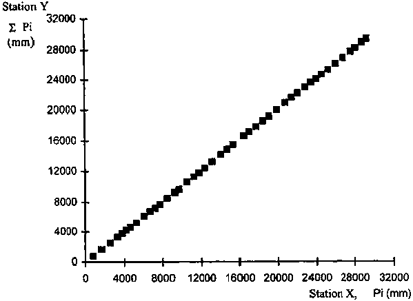
FIGURE 4.7. Double mass after correction of data set Y (case of Figure 4.3)
8. Compute the corrected estimates of the weather variables Yi by solving equation (4-24) for Yi.
Figure 4.7 illustrates the double mass after correction of subset Y in Figure 4.3, where the cumulative sums now follow a straight line.
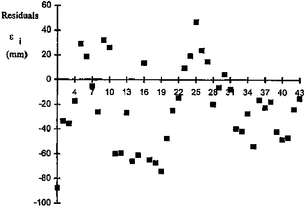
Figure 4.8 is a plot of the corresponding residuals, which now follow a normal distribution. Similar verification can be easily made by the user. This procedure can be easily applied using a spreadsheet computation and graphical packages that are currently available.
FIGURE 4.8. Residuals of the double mass after correction of data set Y (compare to Figure 4.4)
SELECTED BIBLIOGRAPHY ON STATISTICAL ANALYSIS
Dubreuil, P. 1974. Initiation à l'analyse hydrologique. Masson & Cie. et ORSTOM, Paris.
Haan, C. T. 1977. Statistical Methods in Hydrology. The Iowa State University Press, Ames.
Kite, G. W. 1988. Frequency and Risk Analyses in Hydrology. Water Resources Publications, Littleton, CO, 257 pp.
Natural Environment Research Council (NERC) 1975. Flood Studies Report, Vol I - Hydrology Studies. Natural Environmental Research Council, London, 550 pp.
NOTATION IN STATISTICAL ANALYSIS
|
a |
regression coefficient |
|
b |
regression coefficient |
|
covxy |
covariance of variables x and y |
|
Ei |
cumulative residuals |
|
i |
number of order of variable xi in the sample |
|
j, k |
number of a variable in a subset |
|
n |
size of the sample |
|
p |
probability |
|
p (x) |
probability distribution density function |
|
r |
correlation coefficient |
|
r2 |
coefficient of determination |
|
sx |
estimate of the standard deviation of the variable x |
|
|
estimate of the variance of the variable x |
|
sy |
estimate of the standard deviation of the variable y |
|
|
estimate of the variance of the variable y |
|
sy, x |
standard deviation of the residuals of y estimated from the regression |
|
X |
random variable |
|
Xi |
value of a variable in a data set |
|
xi |
random variable |
|
|
estimated value for the variable x with probability of non excedance p |
|
|
estimate of the mean, or mean of a sample of the random variable xi |
|
Y |
transformed variable from X |
|
Yi |
value of a variable in a data set |
|
yi |
random variable |
|
|
value of yi estimated from the regression |
|
|
estimate of the mean, or mean of a sample of the random variable yi |
|
Z |
standard normal variable |
|
zp |
value of the standard normal variable for the probability p |
|
e i |
residuals of y estimated from the regression |
|
m |
mean of a population |
|
s |
standard deviation of a population |