The preceding analysis has presented some preliminary estimates of the economic rent from roundwood production in Suriname. These have been calculated based on current levels of efficiency in the roundwood production sector and using roundwood prices from the upper end of the range of prices currently obtained in Suriname. There are two broad ways in which economic rent could be increased and, consequently, forest charges could be raised in the future:
improvements in the efficiency of forest operations; and
increases in the price of delivered roundwood.
A brief description of the scope for increasing profitability in each of these areas is given below.
Improvements in the efficiency of forest operations
The three main ways in which the efficiency of forest operations could be improved are through:
economies of scale - i.e. encouraging forest concessionaires to operate at a scale that allows them to achieve greater levels of capital utilisation and, consequently, lower unit production costs;
improvements in the efficiency of forest utilisation - i.e. encouraging forest concessionaires to take all commercial standing timber available during each harvesting operation and improve the harvesting efficiency (i.e. reduce harvesting waste during operations); and
investment in work planning and appropriate technology - i.e. increasing the efficiency at each stage of the production cycle and lowering operational costs, through investment in more appropriate technology and better work planning.
In the case of the latter, it is believed that skidding and transportation are the two parts of the roundwood production process where the greatest increases in productivity could be achieved.
Economies of scale
As noted above, current forest operations in Suriname are typically small-scale and the average size of forest concessions in Suriname is quite small, particularly in comparison to other tropical countries. Mitchell (1998a), for example, reports that the average size of former forest concessions in Suriname was just under 12,000 ha. Some forest concessionaires have more than one forest concession, but these are not always close to one another and can not usually therefore, be treated as one management unit. The average size of Incidental Cutting Licences (ICL) and Community Forest (HKV) areas is even less than this - generally around 4,000 ha to 5,000 ha. These areas are currently very important as a source of wood supply because of the slow rate at which new forest concessions have been issued. The few new forest concessions that have been issued are generally larger and the average size of such concessions is currently just under 60,000 ha.
Larger forest concessions should result in lower production costs because they allow machines to be used more efficiently and spend less time idle (i.e. greater capital utilisation) and because any fixed costs will be spread over a greater volume of production.
Capital utilisation. Different pieces of forest machinery operate at different rates of productivity. For example, without any breaks, a chainsaw crew might only be able to cut four trees or around 8 m3 per hour, but a loader can load around 60 m3 or more per hour. Skidders can move at least 5 - 10 m3 per hour, depending on the length and layout of skid trails and the amount of skid trail that each machine has to construct during skidding operations. Similarly, the productivity of timber lorries depends upon the type and capacity of lorries used and the length of the journey from the forest to the processing plant.
With small forest concessions, the rate of productivity achieved at each stage of production is limited by the combination of machinery with high and low rates of productivity (i.e. "bottlenecks" occur at certain stages of the production process). For example, an annual cutting programme of 4,000 m3 would keep one skidder fully employed at current levels of efficiency in Suriname. This level of production would also keep one 20 tonne timber truck fully employed (on an 85 km haul). However, this level of production would only keep the chainsaw crew employed for 60% of their time and utilisation of a loader would be very low (only about 8%). Small-scale operators resolve the problem of what to do about loading timber either by add-hoc means (e.g. driving lorries into trenches that they have dug and pushing the logs on with a skidder) or by hiring contractors to load timber. (This is cheaper than owning a loader, but is still more expensive than if the scale of operations could justify the full-time employment of a proper forest loader). It is generally the case therefore, that forest operations in Suriname are limited by the number of skidders available (usually only one for most forest operators) and operations proceed at a speed determined by this piece of equipment.
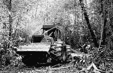
Figure 12 The forest skidder is generally the most heavily utilised piece of equipment in forest operations in Suriname
Besides the problem of mixing different pieces of machinery with different output rates, there is also generally low utilisation of machinery due to the low number of hours that machines are actually available for work in the forestry sector in Suriname. Data collected from forest concessionaires in Suriname (Whiteman, 1999b) suggested that many of them only work for 8 hours per day and 170 days per year, with an average machine availability of 75% (i.e. out of this time, machines are, on average, broken down or out of service for 25% of the time). All three of these factors are low compared with what is achieved in other tropical countries. In Indonesia for example, a 10 hour working day is standard in the forestry sector, with 250 working days per year. Machine availability is 75% or higher, depending on the quality of forest management in each forest concession. This gives a total of 1,500 available working hours per year compared to a figure of just over 1,000 available working hours per year in Suriname.
In order to compare the difference in production costs between the current scale of operations and what could be achieved with greater economies of scale and longer working hours, the roundwood production cost model (Whiteman, 1999a) was used to examine how costs might be reduced with a larger scale of operations, cutting at a greater intensity over a larger area and with more working hours per year. The results of the comparison are given in Table 19.
Table 19 A comparison of production costs and economic rent at the current typical scale of operations in Suriname and with a larger forest operation
|
Production parameters at current scale of operations |
Production parameters with a large scale operation |
|||||||||||||||
|
Forest parameters |
||||||||||||||||
|
Forest concession area |
12,000 ha |
25,000 ha |
||||||||||||||
|
Annual cutting area |
240 ha |
1,000 ha |
||||||||||||||
|
Harvesting intensity |
15 m3 |
20 m3 |
||||||||||||||
|
Annual roundwood production |
3,600 m3 |
20,000 m3 |
||||||||||||||
|
Transport and skidding parameters |
||||||||||||||||
|
One-way transport distance |
85 km |
85 km |
||||||||||||||
|
Skid trail density |
245 m/ha |
245 m/ha |
||||||||||||||
|
Skidding indirectness factor |
82% |
82% |
||||||||||||||
|
Average skidding distance |
910 m |
910 m |
||||||||||||||
|
Production activity |
Machinery and |
Amount |
Machinery and |
Amount |
||||||||||||
|
utilisation |
in Sf |
in US$ |
utilisation |
in Sf |
in US$ |
|||||||||||
|
Felling |
1 felling crew @ 95% utilisation |
1,800/m3 |
1.35/m3 |
3 felling crews @ 95% utilisation |
1,800/m3 |
1.35/m3 |
||||||||||
|
Skid trail construction |
N/A |
N/A |
N/A |
1 D6 bulldozer @ 98% utilisation |
2,850/m3 |
2.10/m3 |
||||||||||
|
Skidding and skid trail construction |
1 wheeled skidder @ 99% utilisation |
12,850/m3 |
9.50/m3 |
2 wheeled skidders @ 98% utilisation |
5,850/m3 |
4.30/m3 |
||||||||||
|
Loading |
1 contract loader @ 7% utilisation |
2,100/m3 |
1.55/m3 |
1 contract loader @ 21% utilisation |
1,300/m3 |
0.95/m3 |
||||||||||
|
Transport |
1 x 20 tonne truck @ 96% utilisation |
11,450/m3 |
8.50/m3 |
3 x 20 tonne trucks @ 97% utilisation |
9,200/m3 |
6.85/m3 |
||||||||||
|
Costs, revenues and rent |
Amount |
Amount |
||||||||||||||
|
in Sf |
in US$ |
in Sf |
in US$ |
|||||||||||||
|
Total production cost |
28,200/m3 |
20.90/m3 |
21,000/m3 |
15.55/m3 |
||||||||||||
|
Average roundwood price |
43,000/m3 |
31.85/m3 |
38,000/m3 |
28.15/m3 |
||||||||||||
|
Economic rent per m3 |
14,800/m3 |
10.95/m3 |
17,000/m3 |
12.60/m3 |
||||||||||||
|
Economic rent per ha per yr |
4,440/ha/year |
3.30/ha/year |
13,600/ha/year |
10.10/ha/year |
||||||||||||
The current scale of operations assumes an average sized forest concession, with a small annual cutting area and low harvesting intensity. In comparison, the large-scale operation assumes a forest concession of just over twice the size of the current average, with an annual cutting area equal to one-twenty-fifth of the total concession area and a harvesting intensity of 20 m3/ha. This would give an annual cut of 20,000 m3 as opposed to 3,600 m3. Skidding and transportation parameters are assumed to be the same in both cases (although there is also scope for improvement there – see Section 5.1.3 Investment in work planning and appropriate technology). Productivity is based on 170 working days per year, an 8 hour working day and 25% machine downtime in the first case and 250 working days per year, a 10 hour working day and 25% machine downtime in the second case. Loading costs calculated by the model have been doubled in both cases as an approximation of the cost of using a contractor to perform this activity.
As the table shows, production costs with more efficient forest operations could be reduced by around Sf 7,000/m3. By increasing the harvesting intensity, the average price paid for roundwood would fall due to the inclusion of second and third grade species in the overall product mix. However, it is likely that the economic rent from production could still be increased by at least Sf 2,000/m3. Perhaps most important however, is the result shown in the last row of the table. By increasing the harvesting intensity and using capital more efficiently, the economic rent from each hectare of forest used for roundwood production could be increased from Sf 4,400/ha/year to Sf 13,600/ha/year, an increase of over 200%. Thus, the more intensive use of the forest would increase its value compared with alternative land uses and allow other areas that are currently used for very extensive forest concessions, to be set aside for conservation purposes or for production in the future. For example, according to these calculations, Surinam's current estimated production of 200,000 m3/year could be met from just ten of these more intensively managed forest concessions with a total area of only 250,000 ha.
Fixed costs. Fixed costs are expenditures that do not vary according to the size of forest concession or the production volume. Examples of fixed costs are the cost of building and maintaining access roads required to link the forest concession to existing roads; the cost of one-off pieces of infrastructure such as quayside facilities; and some components of plan production costs. Some other items of expenditure can be considered as similar to fixed costs in that their cost does not increase strictly in proportion to the size of forest concession or production volume. For example, the cost of a forest inventory for a 100,000 ha forest concession might only be 50% higher than the cost of an inventory for a 50,000 ha concession. Forest camp infrastructure (e.g. accommodation buildings and workshops) and pieces of machinery with very high levels of potential output (e.g. a forest loader or road building bulldozer) can be considered as having cost characteristics that are similar to fixed costs.
Larger forest operations have lower overall production costs because fixed costs will be spread over a greater level of production. For example, if the cost of maintaining an access road were Sf 1,000,000 per year, this would add Sf 1,000/m3 to the total roundwood production cost with an annual production volume of 1,000 m3, but only Sf 50/m3 with an annual production volume of 20,000 m3. The effect of scale of operations on fixed costs is shown in Figure 13. Basically, the cost per m3 of expenditure on fixed factors of production will halve each time that production is doubled.
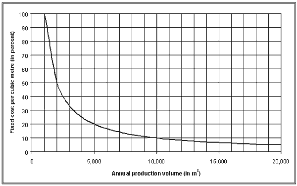
Figure 13 The effect of scale of operations on fixed costs
The impact of fixed costs on total production costs at the current scale of operations in Suriname is not that important at the moment because most forest concessionaires do not invest much in fixed factors of production. For example, road building, forest inventory and planning operations and the construction of forest camp infrastructure are all activities with significant fixed cost components, but are uncommon outside of the few large forest concessions currently operating in Suriname. However, it can be expected that investment in some of these areas (e.g. forest inventory and planning) will be necessary if the country is to move towards a more sustainable forest management system. Investment in roads and forest camp infrastructure will also be required if forest harvesting moves into remoter parts of the interior of the country. Therefore, it is likely that this argument for increasing the average size of forest concessions in Suriname may become stronger in the future.
Improvements in the efficiency of forest utilisation
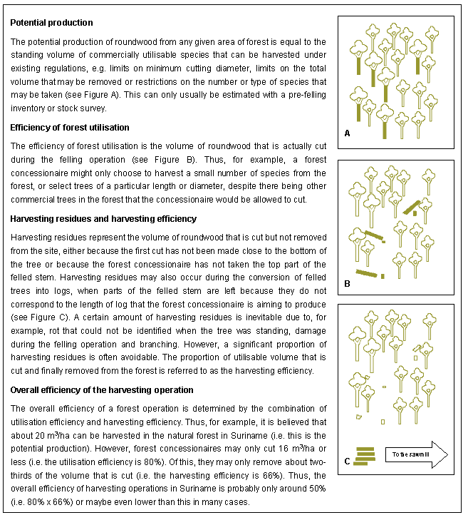
The current efficiency of forest utilisation in Suriname is believed to be very low (see Box 3). There are likely to be two reasons for this:
creaming (sometimes called high grading), or the selection of only the best trees for harvesting during the harvesting operation; and
poor harvesting practices.
Improvements in forest utilisation efficiency could therefore, reduce production costs and benefit the forests of Suriname in other ways.
Creaming. Creaming occurs where forest concessionaires cut only a proportion of the trees that they could during a harvesting operation. This is usually a deliberate decision based on the quality of available trees or due to limited markets for some of the less attractive species that they could potentially cut. It may also occur accidentally if the forest concessionaire has not carried-out a comprehensive survey of all the potentially commercial trees in the forest stand that they are harvesting. Creaming is encouraged wherever forest concessionaires are only charged for the volume of roundwood that they remove from the forest.
The FAO Forest Inventory (FAO, 1974) identified: 52 commercial species; 48 potentially commercial species and 24 possibly commercial species in the natural forests of Suriname. Some species from the latter two groups are now harvested in significant volumes. However, Bruynzeel appears to be the only company currently harvesting a wide range of species (around 20 out of a possible total of 124) although some of the new foreign-controlled logging operations may also be harvesting many different species. In contrast, most small and medium-sized forest operations only tend to take the six to ten most highly valued species. Consequently, it is suspected that the current harvesting intensity might be only 16 m3/ha on average in Suriname and possibly as low as 12 m3/ha in many forest concessions.
There are two main benefits of increasing the volume that is taken from each hectare of forest. Firstly, a higher harvesting intensity will reduce the average production cost due to better capital utilisation and lower fixed costs. For example, at the scale of the felling block, the cost of skid trail construction can be considered as largely a fixed cost. In other words, if it costs Sf 75,000/ha to construct skid trails to remove 15 m3/ha, this would be equal to a cost of Sf 5,000/m3. But, the cost of skid trail construction to remove 20 m3/ha might only be a little more than this, say Sf 80,000/ha, giving a cost of only Sf 4,000/m3. (In other words, very little additional skid trail is required to extract the extra 5 m3/ha). The second benefit of increasing the harvesting intensity is that it will increase the revenue and, consequently, economic rent from production per hectare of forest used for production (both of these arguments are similar to those presented in the previous section). This latter point matters less to the forest concessionaire, but is very important to the forestry administration. Overall, it is possible that increasing harvesting intensity could reduce production costs per m3 by up to Sf 1,000/m3 due to the reasons outlined above.
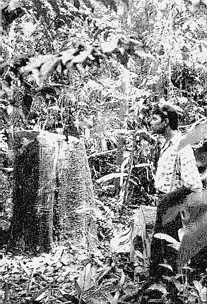
Harvesting practices. Poor harvesting practices include cutting the tree too high (see Figure 14) and leaving utilisable volume from the tops of trees after cutting (often, only one log is cut from each felled tree when, in some cases, it would be possible to cut a second or even a third log). Poor harvesting practices result in low harvesting efficiency or high levels of harvesting waste and can result in increased waste in other ways if, for example, they often lead to breakage or other damage to the log during the felling operation. In addition to the direct impact of poor harvesting practices on utilisable volume, poor practices also increase the probability of accidents during the harvesting operation and can cause substantial damage to the forest remaining after the harvesting operation.
Box 3 Examples of inefficiency in forest utilisation during the harvesting process
Several examples of poor harvesting practices were observed during site visits to forest concessions in Suriname. Consequently, there are likely to be a number of ways in which harvesting practices could be improved, with subsequent improvements in efficiency and production costs. One common practice noted in Suriname was the felling of trees at head height rather than at the base of the trees and this will be examined to show how improved harvesting practices could lead to lower production costs.
The bottom 1.5 metres of a typical standing tree of a commercial size (say 50 cm dbh) and species in Suriname contains up to 0.3 m3 of utilisable timber. Given that the average log size cut and extracted from the forest in Suriname is currently believed to be about 2 m3, this represents about 13% of the potential log volume that is left in the stump when trees are cut at this height (see Figure 14). Admittedly, it does take slightly more time to trim buttresses and fell a tree at the base, but the increased cost of cutting a tree in such a way is likely to be negligible. Similarly, it is unlikely that such a marginal increase in the length of logs extracted from the forest would increase extraction and loading costs significantly. Consequently, an improvement in felling practices that would lead to cutting trees at the base could increase production volume by 13% at little or no extra cost. Alternatively, to put it another way, this could result in an overall reduction in total roundwood production costs of up to Sf 2,200/m3.
Figure 14 An example of poor harvesting practices in a forest concession in Suriname
Investment in work planning and appropriate technology
The final area where significant cost savings could be made is in better work planning and the use of appropriate technology during the roundwood production process. There is probably the greatest scope for improvement in two parts of the process: skidding and the transport of logs from the forest to the mill.
Skidding practices. To a large extent, the average skidding distance determines the average cost of skidding in a forest operation. With longer skid trails, skidding takes more time and requires more fuel to get the roundwood from the forest to the road. If skid trails are very long and poorly laid-out, skidders also produce less total output each day (leading to greater capital costs per m3 of output) and spend more time on skid trail construction. In addition to low levels of efficiency, long skid trails can also result in significant site disturbance, higher skidder repair and maintenance costs and more damage to the remaining forest crop.
The average skidding distance depends upon two factors: the road density and the skid-trail indirectness factor (see Box 4). As the equation in Box 4 shows, the average skidding distance decreases as the road density (or length of roads per ha) in the forest increases. However, increasing the road density requires a higher level of expenditure on road building. Consequently, the optimal road density can be calculated as the amount of road building that minimises the sum of skidding and road building costs (see Figure 15).
The second factor that affects the average length of skid trails, the skidding indirectness factor, depends upon site conditions and the layout of skid-trails. Well planned skid-trails (that attempt to reach all felled trees in as short a distance as possible) can be significantly shorter than unplanned skid trails. Based on field observations and discussions with forest managers, it was observed that skid trails in Suriname currently tend to be very indirect, following roughly the path taken by tree spotters as they work through the forest identifying the location of commercial trees. If this information was put onto simple plans or maps, much shorter skid trails could often be planned using, for example, a main trail roughly up the middle of each section of forest to be harvested and short spurs, or the winch on the skidder, to pull felled trees on to the main trail. This would shorten the average skidding distance and result in lower costs and less damage to the forest.
Box 4 The calculation of average skidding distance from road density and the indirectness factor
|
The calculation of average skidding distance from road density and the skidding indirectness factor is explained below. The average theoretical skidding distance The easiest way to visualise the calculation of the average theoretical skidding distance from road density is to think of strips of forest served by skid trails leading on to forest roads. Thus, for example, assuming that main skid trails are 200m apart and that road density is 5 m/ha, two main skid trails, one off each side of a 200m segment of forest road, must serve 40 ha (200 m divided by 5 m/ha). The length of road is the length of one side of the strip of forest served by the road so, from the total area (i.e. 40 ha), the length of the strip can be determined. One hectare equals 10,000 m2, so 40 ha equals 400,000 m2 and, if the road side is 200 m long, the length of the strip of forest served by the road must be 400,000 m2 divided by 200 m, which equals 2,000 m. This is shown in the figure below:
The total length of the strip on each side of the road is 1,000 m, so the centre of the strip on each side of the road and, hence, the average theoretical skidding distance is 1,000 m divided by two, which equals 500 m. More generally, the theoretical skidding distance can be calculated using the formula below: Theoretical skidding = 2,500 . distance (in metres) road density (in m/ha) The skidding indirectness factor In reality of course, it is very difficult to achieve the average theoretical skidding distance because site factors such as steep areas and streams make it necessary to deviate from the most efficient route to each tree. Poor skid trail layout can also lead to a large amount of deviation from the most efficient route. Therefore, the above calculation is usually multiplied by an indirectness factor to take into account these considerations. A model was constructed for this study to examine the impacts of stocking, skid trail layout and road density on skidding length, which suggested that a high level of indirectness (82%) would probably be typical in forest concessions in Suriname. The final skidding distance is therefore, equal to the theoretical average skidding distance plus this factor which, with a road density of 5 m/ha, equals 500 m x (100% + 82%), which equals 910 m. |
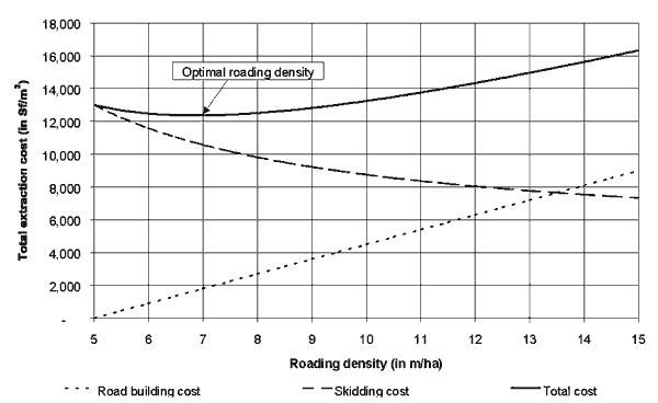
Figure 15 Calculation of the optimal road density as the minimum of skidding and road building costs
In order to examine the scope for reducing skidding costs, a simple model was constructed to estimate the effect of better skid trail layout on the skidding indirectness factor and, consequently, the overall skidding distance. This compared the average length of skid trails and amount of skid trail construction required under two different options:
skid trails going to each tree following root and branch pattern that minimises the distance between each cut tree and all previously cut trees as the skidder works further into the forest (an approximation of current skid-trial layout); and
a main skid trail up the centre of each strip of forest to be harvested, with use of the winch to pull-in cut trees that are less than 25 m away from the skid trail and short spurs to reach cut trees that are further away than this (as an approximation of a more efficient skid trail design).
The model was run for three different levels of forest stocking or harvesting intensity, three different levels of road density and for skid trails 100 m apart and 200 m apart. The model was run for 100 simulations of each of these combinations and the average results for each of these combinations are shown in Table 20 and Table 21.
Table 20 Skid trail construction and average skidding length with unplanned and planned skid trails (100 metres apart) at various levels of road density and stocking levels
|
Road |
Stocking |
Unplanned skid trails |
Planned skid trails |
||||||
|
Density (m/ha) |
Level (m3/ha) |
Skid trail |
Average skid |
Indirect- ness |
Skid trail |
Average skid distance (in metres) |
Indirect -ness |
||
|
density (m/ha) |
distance (m) |
factor (%) |
density (m/ha) |
by winching |
by skidding |
In total |
factor (%) |
||
|
12 |
215 |
405 |
62 |
49 |
19 |
291 |
310 |
24 |
|
|
10.0 |
16 |
249 |
415 |
66 |
63 |
19 |
293 |
312 |
25 |
|
20 |
277 |
418 |
67 |
78 |
19 |
291 |
310 |
24 |
|
|
12 |
217 |
529 |
59 |
48 |
19 |
389 |
408 |
23 |
|
|
7.5 |
16 |
248 |
539 |
62 |
63 |
19 |
391 |
410 |
23 |
|
20 |
281 |
562 |
69 |
78 |
19 |
390 |
409 |
23 |
|
|
12 |
221 |
794 |
59 |
47 |
19 |
581 |
600 |
20 |
|
|
5.0 |
16 |
252 |
812 |
62 |
61 |
19 |
578 |
597 |
19 |
|
20 |
280 |
815 |
63 |
76 |
19 |
577 |
596 |
19 |
|
Table 21 Skid trail construction and average skidding length with unplanned and planned skid trails (200 metres apart) at various levels of road density and stocking levels
|
Road |
Stocking |
Unplanned skid trails |
Planned skid trails |
||||||
|
Density (m/ha) |
Level (m3/ha) |
Skid trail |
Average skid |
Indirect- ness |
Skid trail |
Average skid distance (in metres) |
Indirect -ness |
||
|
density (m/ha) |
distance (m) |
factor (%) |
density (m/ha) |
by winching |
by skidding |
In total |
factor (%) |
||
|
12 |
214 |
473 |
89 |
195 |
22 |
315 |
337 |
35 |
|
|
10.0 |
16 |
247 |
484 |
94 |
264 |
22 |
320 |
342 |
37 |
|
20 |
275 |
493 |
97 |
328 |
22 |
322 |
344 |
38 |
|
|
12 |
213 |
608 |
83 |
190 |
22 |
408 |
430 |
29 |
|
|
7.5 |
16 |
245 |
627 |
88 |
265 |
22 |
417 |
439 |
32 |
|
20 |
273 |
616 |
85 |
327 |
22 |
415 |
437 |
31 |
|
|
12 |
212 |
883 |
77 |
195 |
22 |
606 |
628 |
26 |
|
|
5.0 |
16 |
245 |
910 |
82 |
265 |
22 |
610 |
632 |
26 |
|
20 |
273 |
919 |
84 |
375 |
22 |
610 |
632 |
26 |
|
Source: Author's own estimates (skidding model results)
The total roundwood production cost figures presented in the previous sections of this report assumed a road density of 5 m/ha, with skid trails 200 m apart. According to the simulation model, this would result in a skid-trail indirectness factor of 82% and an average skidding distance of 910 m. This is a very long skidding distance compared with current forestry practice in many other tropical countries. However, it was confirmed, during several field trips and interviews with forest concessionaires, that average skidding distances of around 1 km are typical of current forestry practices in Suriname.
As the tables show, the model suggests that varying the road density and skid-trail design would have the following effects:
distance between skid-trails
the average skidding distance would be slightly higher (+5% to +15%) with skid trails 200 m apart than with skid trails 100 m apart;
average skid trail construction, with planned skid trails, is much higher (+300% to +400%) with skid trails 200 m apart than with skid trails 100 m apart, due to the high number and length of side trails that would be required (it should be noted however, that this is largely a result of the simplicity of the model – in reality, it would be expected that a wider distance between skid trails would result in more skid trail construction overall, but not by as much as the model suggests);
if there is no planning of skid trails, the average amount of skid trails constructed in the forest is not affected by the distance between skid trails;
stocking level and harvesting intensity
the average skidding distance is slightly higher (up to +5%) with higher stocking in the case of unplanned skid trails, but with planned skid trails the difference is insignificant;
average skid trail construction is higher with higher stocking;
road density
the average skidding distance is roughly halved if the road density doubles, but less so if skid trails are unplanned and 200 m apart;
average skid trail construction is unaffected by the level of road density;
planned skid trail layout
planned skid trails result in a significant reduction (-30% to -35%) in the average skidding distance compared to unplanned skid-trails;
planned skid trails result in a significant reduction (-70% to -80%) in skid trail construction compared to unplanned skid-trails, if skid-trails are 100 m apart;
if skid-trails are 200 m apart, skid trail construction is not significantly different with planned skid trails compared to unplanned skid-trails (but, as noted above, this is largely a result of the simplicity of the model used here – in reality there are nearly always likely to be some savings in skid trail construction with proper planning); and
generally, the benefits from planned skid trails are much greater if the skid trails are 100 m apart.
In conclusion, it would seem that, with skid-trails 100 m apart, planned skid-trails could reduce the skid-trail indirectness factor from around 80% to around 20%, with consequent savings in skidding costs.
The next stage of this analysis was to examine what the cost saving would be with planned skid trails and an optimal level of road density. This was calculated using the roundwood production cost model (Whiteman, 1999a) and data on the cost of skidding and road building collected in Suriname (Whiteman, 1999b). It is true that proper skid-trail layout requires a certain amount of training, a pre-felling inventory, a simple map and some planning of the skid trail layout, which would lead to greater expenditure in this area. However, no data is currently available about how much this might cost. Therefore, it has been assumed that these costs would be negligible in the comparison presented below.