The study of fish growth and of phenomena related to growth such as maturation, migration, food and feeding habits is central to fishery biology. Indeed, it is largely with growth studies that fishery biology established itself as a field of its own by the end of the last century.
Knowledge of how the fishes of a given stock grow is essential for most stock assessment purposes, both in the tropics and elsewhere, since it is the growth of individual fishes which provide from year to year the catch taken by a fishery.
For practical reasons, the available information on the growth of fishes of a given stock is generally reduced to and expressed by means of a single equation, such as the Von Bertalanffy Growth Formula (VBGF), the simplest version of which has the form
Lt = L∞(l-e-K(t-t)o) | (9) |
Where L∞ is the mean length the fish would reach if they were to grow to a very old age (indefinitely, in fact)
K is a growth coefficient
to is the “age” the fish would have had length zero if they had always grown according to the equation (to generally has a negative value)
and where
Lt is the length at age t.
The biological data which can be used to obtain information (“growth data”) from which growth parameters can be estimated are of three basic types:
In spite of frequent criticism, the methods for the analysis of length frequency data have found, in the tropics, wider applications than the study of skeletal parts, while tagging studies have generally been underutilized. The reason for this is that it is generally easier to analyse length frequency data than to study skeletal parts and that much less equipment is needed; this also applies to the comparison with tagging studies.
Methods for the Analysis of Length-Frequency Data
The methods currently in use for the analysis of length-frequency data all find their origin in the work of Pertersen (1892 and subsequent years). Traditionally, however, the name of Petersen has been associated with only one of the specific approaches commonly used, such that we may distinguish three methods for the analysis of length-frequency data.
With the “Petersen method”, assumptions are made as to the time interval separating the various peaks of one length-frequency sample, these peaks being assumed to represent distinct age groups (Figure 3).
With the second method, assumptions are made as to which of the peaks can be inter- connected that belong to various samples arranged sequentially in time (Figure 4).
As Figures 3 and 4 show, the methods are quite subjective in the sense that several options are available for attributing ages to the various age groups (in Figure 3) or for interconnecting peaks (in Figure 4). Thus, both the “Petersen method” and the “modal class progression analysis” are often fraught with uncertainties. Some of these uncertainties can be overcome, however, by combining the two methods to an “integrated method” in which an attempt is made to draw a growth curve (e.g., with a curved ruler) directly upon the length-frequency samples sequentially arranged in time (as in Figure 5) or onto the same sample repeated over and over along the time axis (as in Figure 6).1 The method is based on the following tenets:
(1) Length growth in fishes is at first rapid, then decreases smoothly and is, for the population as a whole, best approximated by a long continuous curve, rather than by several, short straight segments.
(2) A single, smooth growth curve interconnecting the majority of the peaks of sequentially arranged length-frequency samples is likely to represent the average growth of the fishes of a given stock.
(3) The growth patterns repeat themselves from year to year (which is also assumed when the “annuli” of otoliths are counted).
Thus, the curve in Figure 5 which interconnects most of the peaks of the 1957 Leiognathus bindus samples of Balan (1967) can be used to estimate the growth parameters of that species of slipmouth. An additional example for the application of the integrated method to length- frequency data of tropical fishes may be given here (Figure 7), pertaining to length-frequency data on Sardinella sirm from the Java Sea. Note that the length-frequency data, as presented by their original authors do not suggest any growth process, while the same data redrawn in the appropriate manner suggest a clear growth pattern and a single major growth curve which, when drawn, can be used to estimate growth parameters in this fish.
This example illustrates once more the major features of the integrated method:
(1) The intervals on the time axis between the various samples must be proportional to the time elapsed between the sampling dates.
(2) The original data must be plotted at least twice, or more along the time axis, which allows for longer, stabilized growth curves to be drawn and for all relevant age groups to be included in one single line.
(3) When several growth curves are drawn (reflecting the production of several broods per year) the various growth curves should have the same shape, and vary only as to their origin.
(4) The scale of the ordinate (length) should start at zero, thus allowing approximate spawning periods to be identified.
(5) Each growth curve must interconnect several peaks. The more peaks a curve inter- connects, the more likely it is to depict the actual growth of the population.
1 When several years' worth of data are available, repeating the sample(s) over and over is obviously superfluous
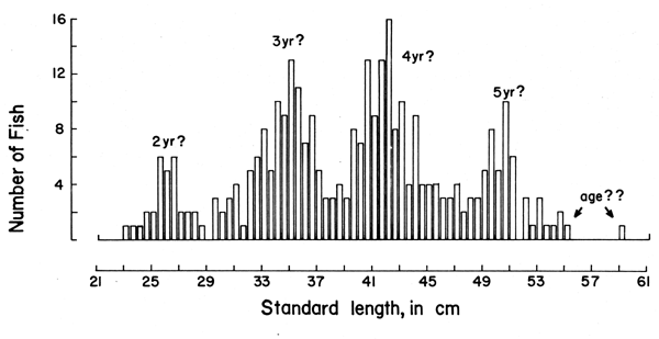
Figure 3 Length-frequency data on the coral trout (Plectropomus leopardus)obtained by Goeden (1978) from Heron Island (Great Barrier Reef, Australia) in October 1977. The “ages” are from Goeden, with question marks added. N = 319
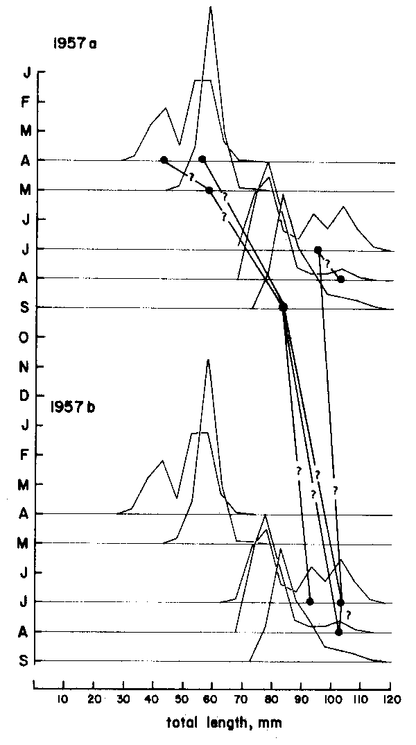
Figure 4 Showing that there are several options for connecting peaks when using the “modal clas progression analysis”. Based on data of Balan (1967), for Leiognathus bindus caught in 1957 off Calicut, India. For numbers included in each samples see Figure 10
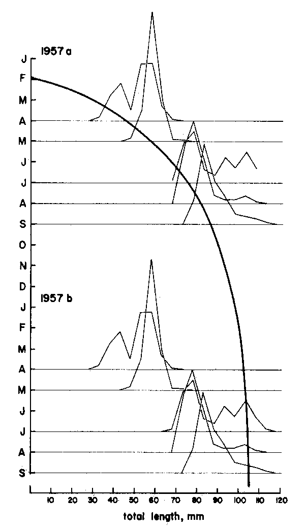
Figure 5 Showing how drawing a single, continuous growth curve onto a series of samples sequentially arranged in time limits the number of available options for connecting peaks to only one single, most probable option. Note repetition of sample sequence over two “years”. Based on data Balan (1967), for leiognathus bindus caught in 1957 off Calicut, India. For numbers included in each sample see Figure 10
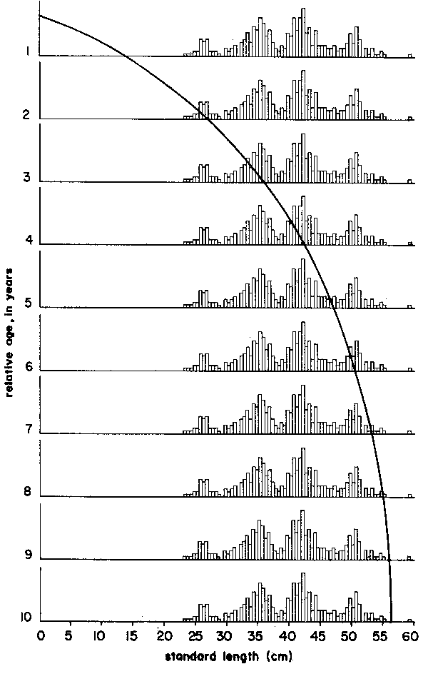
Figure 6 Showing how the single sample of Figure 3 when repeated over and over along the time axis can be fitted by eye, with a single continuous and smooth growth curve. Note that from “age” 4 on, the curves provide an interpretation of the growth of Plectropomus leopardus different from that given by Goeden, 1978 (see Figure 3 and text)
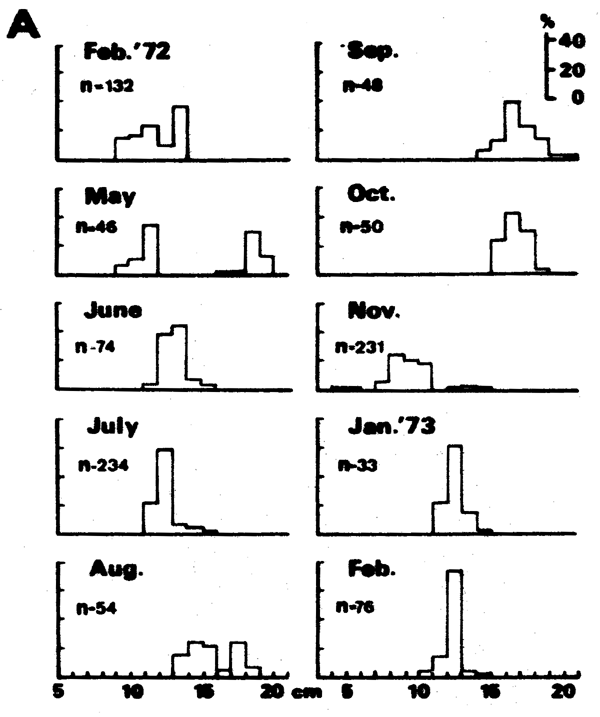

Figure 7 A - Length-frequency data on Sardinella sirm as presented by their original authors (Burhanuddin et al., 1974)
B - The same data, redrawn according to the integrated method (see text)
(6) The modal lengths corresponding to various ages (starting from an arbitrary age) can be read off the curve at regular time intervals, and may be then used to determine the growth parameters with a method as simple as a Ford-Walford Plot (see further below).
It is my experience that length-frequency data published in the literature or available in the form of unpublished manuscripts are generally underutilized, especially in the tropics. More often than not, no attempt is made to extract growth parameters from length-frequency data even when these are eminently suitable to such treatment, as shown in Figures 4 to 7. Also, I believe that the danger of obtaining completely erroneous growth parameters from length-frequency data is generally overstated, at least as far as small tropical fishes are concerned. In fact, the integrated method, as presented here makes it quite hard to trace “wrong” growth curves, and the parameters obtained from such curves will describe the growth of at least the exploited part of a population well enough for most purposes.
| Exercise: | Plot length-frequency data of your own (or taken from the literature), trace most probable growth curve(s) according to the integrated method and read off the lengths at monthly intervals. |
Methods for Obtaining Growth Parameters from Length-at-Age Data
The method most commonly used for estimating the parameters L∞ and K of the VBGF is the “Ford-Walford Plot” which essentially consists of a rewritten version of the VBGF of the form
Lt+1 = a + bLt | (10) |
| where L∞ = a ÷ 1-b | (11a) |
| and K = -loge b | (11b) |
and where Lt and Lt+1 pertain to lengths separated by a constant time interval (1 = year, month, week, etc.). Table 3 below shows how length-at-age data should be rearranged for use with a Ford-Walford Plot.
| Age (y) | L (cm) | Rearrangement for Ford-Walford Plot | |
|---|---|---|---|
| 1 | 35 | Lt (x) | Lt+1 (y) |
| 2 | 55 | 35 | 55 |
| 3 | 75 | 55 | 75 |
| 4 | 90 | 75 | 90 |
| 5 | 105 | 90 | 105 |
| 6 | 115 | 105 | 115 |
The data provide estimates of a = 26.17 and b = 0.859, from which, using Equations 11a and 11b, we estimate L∞ = 186 and K = 0.152.
| Exercise: | (a) | Draw a Ford-Walford Plot with the data of Table 3 and estimate L∞ from the intersection of the Plot with the line Lt+1 = Lt |
| (b) | Estimate the growth parameters L∞ and K for Plectropomus leopardus, Leiognathus bindus and Sardinella sirm using the growth curves in Figures 5, 6 and 7, Ford-Waldford Plots and the regression technique for estimating the a and b values. |
An Alternative Method for Estimating Growth Parameters
When continuous growth lines (such as in Figures 5, 6 and 7) cannot be traced, or when only tagging and recapture data are available, the growth data obtained cannot be used in conjunction with a Ford-Walford Plot. In such cases, the “Gulland and Holt Plot” may be used, which provides estimates of L∞ and K through the feature that

where  , and wher L1 and L2 are successive lengths, pertaining to times t1 and
t2, respectively.
Table 4 and Figure 8 give an example of data of this kind, which are typically obtained from tagging studies. The method, however, also allows for the use of size-at-age data, at equal or unequal intervals granted the values of (t2 - t1) stay small in relation to the longevity of the fish (Gulland and Holt, 1959).
Equation 12 it will be noted, has the form of a linear regression with

the intercept (a) and slope (b), which provide values of K and L∞ through the relationships
K = -b
and 
At times, it will happen that the method does not provide reasonable parameter estimates.
This will occur most often when the  data are too close to each other (Figure 9). In such
a case, a set value of the asymptotic length may be used in connexion with the means of all
 values (
 ) and of all
  values (
 ) to obtain an estimate of K through

This method, called “forced” Gulland and Holt Plot, allows in fact for a rough first estimate of K even when only one pair of x and y values are available.
| Number | L1 (cm) | L2 | Days out |
|---|---|---|---|
| 1 | 9.7 | 10.2 | 53 |
| 2 | 10.5 | 10.9 | 33 |
| 3 | 10.9 | 11.8 | 108 |
| 4 | 11.1 | 12.0 | 102 |
| 5 | 12.4 | 15.5 | 272 |
| 6 | 12.8 | 13.6 | 48 |
| 7 | 14.0 | 14.3 | 53 |
| 8 | 16.1 | 16.4 | 73 |
| 9 | 16.3 | 16.5 | 63 |
| 10 | 17.0 | 17.2 | 106 |
| 11 | 17.7 | 18.0 | 111 |
| Number | L1 (cm) | L2 | Days out |  | cm/day |
|---|---|---|---|---|---|
| 1 | 14.0 | 16.9 | 48 | 15.45 | 0.0604 |
| 2 | 20.8 | 27.6 | 189 | 24.2 | 0.0360 |
| 3 | 24.8 | 26.5 | 48 | 25.65 | 0.0354 |
means:  = 21.77 = 21.77  = 0.0439 = 0.0439 | |||||
1 Adapted from Table 17 of Randall (1962)
The use of a set value for the asymptotic length is here coded L(∞), to distinguish it from values of L∞ obtained from the growth data themselves. Reasonable values of L(∞) can generally be obtained from the empirical relationship

where Lmax is the length of the largest fish reported from a well sampled stock, if at all possible, taken at a time when exploitation was still low.
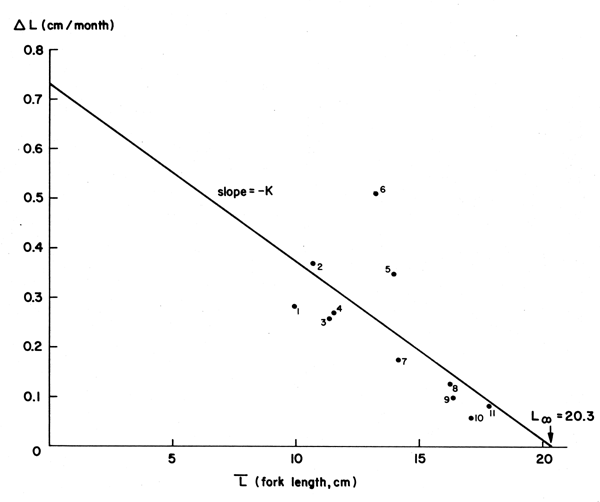
Figure 8 Showing a “Gulland and Holt Plot” of data on the ocean surgeon fish (Acanthurus bahianus) (see Table 4 and text)
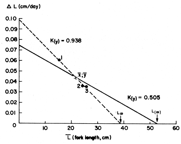
Figure 9 Showing a “Gulland and Holt Plot” and a “forced Gulland and Holt Plot” for the queen parrot fish (Scarus vetula). Based on data of Table 5; see text
The Gulland and Holt Plot does not allow for the estimation of the third parameter of the VBGF, to. When this parameter is necessary (e.g., when a certain age is to be attributed to a certain length) a rough estimate of to may be obtained from the empirical relationship.
| log10(-to) = -0.3922 -0.2752 log10 L∞ -1.038 log10 K | (17) |
derived in Pauly (1979a) from 153 triplets of to, L∞ (total length, in cm) and K (annual basis) selected from my compilation of length growth parameters (Pauly, 1978a) such as to cover a wide diversity of taxa and size.
| Exercise: | Calculate values of L∞, K from the data of Table 6 (see Figure 10) on Leiognathus bindus for the years 1956, 1957 and 1958 using the Gulland and Holt Plot and obtain a rough estimate of to, using Equation 17. |
| Segment number | h |  | Segment number | h |  |
|---|---|---|---|---|---|
| 1 | 0.50 | 9.0 | 7 | 1.00 | 6.7 |
| 2 | 0.50 | 9.4 | 8 | 0.50 | 8.4 |
| 3 | 1.23 | 7.4 | 9 | 0.50 | 8.0 |
| 4 | 1.00 | 9.7 | 10 | 0.50 | 10.0 |
| 5 | 0.30 | 10.4 | 11 | 0.50 | 9.2 |
| 6 | 1.50 | 5.0 | 12 | 1.00 | 6.2 |
| 13 | 0.50 | 7.7 |