Introduction
In fishery biology, the most useful manner of expressing the decay (=decrease) of an age group of fishes through time is by means of exponential rates. These rates, of which three are normally defined, are given in the following two expressions:
NT = No · e-Zt | (18) |
where No is the (initial) number of fishes at time t = o, and Nt is the number of remaining fishes at the end of time t, Z being the instantaneous rate of total mortality. An advantage of instantaneous rates is that they can be added or subtracted. Thus we have
Z = M + F | (19) |
where M is the instantaneous rate of natural mortality and F the instantaneous rate of fishing mortality (see Figure 11). Obviously, when
F = 0 then, Z = M | (20) |
which means that natural and total mortality have the same value when there is no fishing (in an unexploited stock).
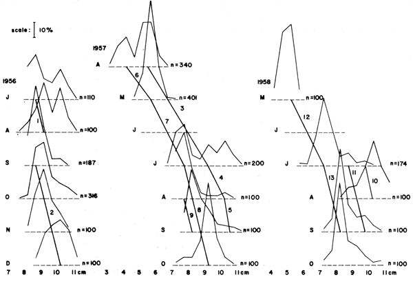
Figure 10 Length-frequency data on the slipmouth Leiognathus bindus caught off Calicut, India in years 1956, 1957 and 1958, with suggested “growth segments” for use with a Gulland and Holt Plot (see Table 6 and text). Based on data of Balan 1967
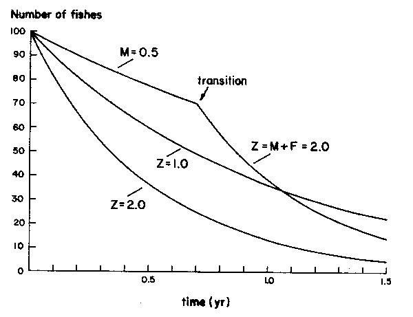
Figure 11 Showing the decrease of a cohort of fishes, over time, starting with 100 fishes at age 0, with 3 levels of mortality
The fishery biologist, as far as mortalities are concerned, has two main jobs:
(a) To estimate the value of Z;
(b) To split - where appropriate - an estimated value of Z into its component parts M and F.
Estimating Total Mortality
Total mortality from the mean size in the catch
(a) When a large number of length-frequency data have been obtained from a given stock,
by a given gear, Z can be estimated from the mean length ( ) in the catch from a given population
by means of

Where L∞ and K are parameters of the von Bertalanffy growth equations,  is the mean length
in the catch, and “L' is the smallest length of animals that are fully represented in catch
samples” (Beverton and Holt 1956).
(b) Another equation which can be used to estimate Z from the mean length in the catch is

where L∞,  , L' and K are defined above while n is the number of fishes used for the estimation
of
  (based on Ssentengo and Larkin 1973). It will be noted that when n is large, the term
n/n+1 tends toward unity and hence can be neglected.1
(c) The equation corresponding to Expression 22 is for weight (when growth is isometric):

where W∞ and K are parameters of the von Bertalanffy growth function for weight growth, which has the form
Wt = W∞ (1-e-K (t-to))3 | (24) |
with  and W' being the weight corresponding to
  and L' as obtained (along with W∞) from a
conversion from length to weight, by means of the appropriate length-weight relationship.
Equation 24 is particularly useful in that it is quite easy to weigh a catch and to
divide it by the number of fish to obtain  .
.
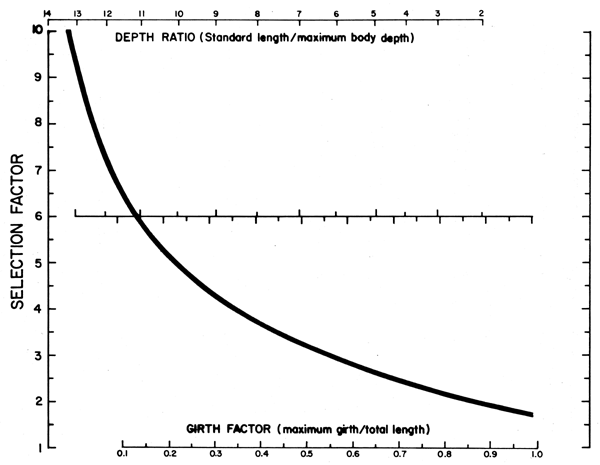
Figure 12 Nomogram for the estimation of the selection factors of fishes from measurements of their body proportions. Based on data in Sinoda et al., 1979 and Meemeskul (1979). Original. (Note: all selection factors estimated by means of this nomogram refer to total length. Hence: SF . mesh size = Lc (total length))
| Year | Effort | n |  | Z1 | Z2 |
|---|---|---|---|---|---|
| 1966 | 2.08 | 4 733 | 13.25 | 2.41 | 2.95 |
| 1967 | 2.08 | 11 902 | 13.01 | 2.69 | 3.24 |
| 1968 | 3.50 | 12 503 | 12.99 | 2.72 | 3.27 |
| 1969 | 3.60 | 9 060 | 13.07 | 2.62 | 3.16 |
| 1970 | 3.80 | 8 132 | 12.37 | 3.73 | 4.29 |
| 1972 | 7.19 | 3 635 | 12.30 | 3.88 | 4.44 |
| 1973 | 9.94 | 10 510 | 12.01 | 4.61 | 5.14 |
| 1974 | 6.06 | 7 960 | 12.60 | 3.30 | 3.85 |
 | 4.87 | 12.70 | 3.25 | 3.79 | |
Constants: L∞ = 20.0; K = 1.16; Lc = 10.0 (Z1 = equation 21; Z2 = equation 22) | |||||
A parameter closely related to L' (see above for definition) is the mean length at first capture (Lc), or the length at which 50% of the animals sampled are retained by the gear.
Lc is normally estimated from selection experiments (see Gulland 1969) which, however, are rather time and resource consuming. To facilitate estimation of Lc, a figure is therefore included which allows for values of Lc to be obtained from attributes of fish that are very easy to obtain, such as the length/depth ratio, or the “girth factor” of fishes (Figure 12).
Figure 12, however, does not allow for a direct estimation of Lc. Rather, once the length/depth ratio or the girth factor have been estimated, Figure 12 is used to estimate a selection factor (SF) such that
Lc = SF · mesh size (of cod end)1 | (25) |
The parameter Lc is used in stock assessment in a number of models, notably that of Beverton and Holt (1966). In cases where “knife-edge” selection occurs (see Beverton and Holt 1966, or Gulland 1969), Lc = L'; generally however, L'> Lc.
1 When the sampling gear is a trawl
Estimating Z by means of a Catch Curve
Another method of estimating Z consists of sampling a multi-aged population of fishes, then plotting the natural logarithm (loge) of the number of fishes in the sample (N) against their respective age (t) or
logeN = a + bt | (26) |
where the value of b, with sign changed, provides an estimate of Z.
Several requirements must be met for the values of -b to be a good estimator of Z. Among these, we may mention:
(a) Only those values of logeN must be included which pertain to age group of fishes fully vulnerable to the gear in question (among other things, the fish must be larger than L' as defined above): This corresponds to using only the “descending part” of a catch curve (see Figure 13).
(b) Recruitment must have been constant within the period covered, or have varied in a random fashion only.
When suitable length-frequency samples are available, a catch curve may also be constructed through previous conversion from length to age by means of a set of growth parameters. Here, however, care must be taken not to include fish whose size is close to that of their asymptotic size, as this may result in their age being grossly over-estimated. This latter feature incidentally makes it imperative that a scatterdiagram be drawn in order to properly identify the section of the catch curve which can be used to estimate Z (Figure 13). It will be noted, also, that since Z is equal to the slope (with sign changed) of the catch curve the real age - which requires an estimate of to - can be here replaced by relative age, i.e., by setting to = 0 (Table 8, Figure 13).
Also, when converting a length-frequency sample to a catch curve, a problem must be considered which doesn't occur when fish have been aged individually. This problem is due to the fact that length growth not being linear, it takes an older fish longer than a younger fish to grow through a given size-group. Put another way, among bigger fish, a given magnitude of size interval (e.g., a l-cm length group) will contain more age groups than among small fish.
Compensating for this “piling-up” effect is, however, quite straightforward and can be achieved, e.g. by rewriting equation (26) as
loge (N/∆t) = a + bt | …(26a) |
where ∆t is the time needed to grow from the lower (t1) to the upper (t2) limit of a given length class, while t is the relative age corresponding to the midrange of the length class in question. The procedure to convert a length-frequency to a length-structured catch curve is illustrated in Table 8 and Fig. 13.
| Class limits | Mid-range2 | N | t13 | t23 | ∆t | Adjusted number per length class logeN/∆t | Mean relative age t3 | Remarks | ||
|---|---|---|---|---|---|---|---|---|---|---|
| Lower2 | Upper2 | |||||||||
6.000 | 6.999 | 6.5 | 3 | 0.510 | 0.612 | 0.102 | 3.38 | 0.56 |  | Not used, ascending part of curve |
7.000 | 7.999 | 7.5 | 143 | 0.612 | 0.720 | 0.109 | 7.18 | 0.67 | ||
8.000 | 8.999 | 8.5 | 271 | 0.721 | 0.837 | 0.116 | 7.76 | 0.78 | ||
9.000 | 9.999 | 9.5 | 318 | 0.837 | 0.961 | 0.125 | 7.84 | 0.90 | ||
10.000 | 10.999 | 10.5 | 416 | 0.961 | 1.096 | 0.134 | 8.04 | 1.03 | ||
11.000 | 11.999 | 11.5 | 488 | 1.096 | 1.242 | 0.146 | 8.11 | 1.17 | ||
12.000 | 12.999 | 12.5 | 614 | 1.242 | 1.402 | 0.160 | 8.25 | 1.32 | ||
13.000 | 13.999 | 13.5 | 613 | 1.402 | 1.579 | 1.777 | 8.15 | 1.49 |  | Portion used for estimating Z |
14.000 | 14.999 | 14.5 | 493 | 1.579 | 0.176 | 1.999 | 7.13 | 1.67 | ||
15.000 | 15.999 | 15.5 | 278 | 1.776 | 1.999 | 0.223 | 7.13 | 1.88 | ||
16.000 | 16.999 | 16.5 | 93 | 2.000 | 2.257 | 0.257 | 5.89 | 2.12 | ||
17.000 | 17.999 | 17.5 | 73 | 2.257 | 2.560 | 0.303 | 5.48 | 2.40 | ||
18.000 | 18.999 | 18.5 | 7 | 2.260 | 2.930 | 0.370 | 2.94 | 2.74 | ||
19.000 | 19.999 | 19.5 | 2 | 2.930 | 3.404 | 0.473 | 1.44 | 3.15 | ||
20.000 | 20.999 | 20.5 | 2 | 3.404 | 4.063 | 0.659 | 1.11 | 3.70 |  | Not used, too close to L∞ |
21.000 | 21.999 | 21.5 | 0 | 4.064 | 5.159 | 1.094 | - | 4.53 | ||
22.000 | 22.999 | 22.5 | 1 | 5.160 | 9.208 | 4.047 | -1.40 | 6.19 | ||
23.000 | 23.999 | 23.5 | 1 | - | - | - | - | |||
1 Form Ziegler (1979) who also gives: L∞ = 23.1 and K = 0.59 and T = 28°C
2 Total length, in cm
3 Computed by means of equation 32, with to = 0
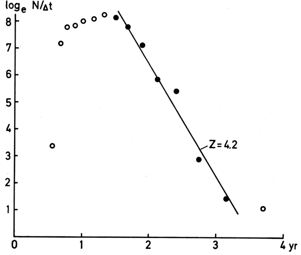
Figure 13. A catch curve based on length converted to age, and corrected for the time needed for the fish to grow through the size classes (see next). Based on the data of Table 8, the regression equation is loge(N∆t) = 14.8 - 4.19t, (r = 0.988), which provides an estimate of Z = 4.2.
Splitting Z into M and F
Splitting Z into M and F by means of a plot of Z on effort
When values of Z are available for several years pertaining to different annual values of effort (f), the value of M can be calculated from
Z = M + qf | (27) |
where q is the “catchability coefficient”, which relates f and fishing mortality (F) through
F = q · f | (28) |
Thus, a series of Z (mean annual) values can be plotted against their corresponding values of f and a straight line fitted to the points by means of linear regression technique. This results in a regression line with the equation
y = a + bx | (29) |
where Z = y and x = f, the slope (b) of which provides an estimate of the catchability coefficient q while the intercept value (a) is an estimate of M (see Figure 14) in which values of Z based on Equations 21 and 22 have been plotted.1
Splitting Z into M and F by means of an independent estimate of M
When only one value of Z is available, or when the available values of Z and f cover too small a range of Z and f values for reasonable values of M and q to be obtained, the catchability coefficient (q) may be estimated through

where  is the mean of the available values of Z (or a single value of Z) and
  is the mean
of the values of f (or a single value of f), M being an independent estimate of natural mortality
(see Table 7 and Figure 14).
Method for Obtaining Independent Estimate of M
It has been demonstrated by various authors that the value of the parameter K of the VBGF in fishes is closely linked with their longevity. This can be demonstrated on the basis of the observation that, generally, in nature, the oldest fishes of a stock grow to reach about 95 percent of their asymptotic length (Taylor, 1962; Beverton, 1963). Thus when we have
Lt = L∞ (1-e-K(t-to)) | (31) |
we also have

1 It will be noted that equation 22 produces estimates of Z which are higher than those obtained using equation 21; Mr. P. Sparre (Danish Institute for Fishery and Marine Research) suggests (pers.comm.) that equation 22 is biased upward.
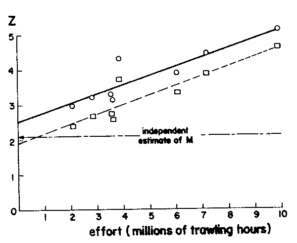
Figure 14 Plots of total mortality (z) on effort (f) to estimate natural mortality and catchability coefficient in
Selaroides leptolepis from the Gulf of Thailand. Based on data in Table 7. The equations are:
Z1 = 1.96 + 0.263f (squares)
Z2 = 2.52 + 0.263f (dots)
or, if we insert 95 percent of L∞ for the oldest fish

thus

where tmax is the longevity of the fishes in question.
That natural mortality should, in fishes, be correlated with longevity, hence with K, seems obvious. Natural mortality should, in fishes, also correlate with size since large fishes should have, as a rule, fewer predators than small fishes.
Natural mortality in fishes can also be demonstrated to be correlated to mean environmental temperature (Pauly, 1978b, 1980a.) These various interrelationships can be expressed for length-growth data by the multiple regression
log10M = -0.0066-0.279 log10L∞ + 0.6543 log10K + 0.4634 log10T | (35) |
and for weight-growth data by
log M = -0.2107-0.0824 log10W∞ + 0.6757 log10K + 0.4687 log10T | (36) |
Where M is the natural mortality in a given stock, L∞ (total length in cm) and W∞ (live weight in g) being the asymptotic size of the fishes of that stock, and K their growth coefficient. The value of T, finally, is the annual mean temperature (in °C) of the water in which the stock in question lives, as obtained, e.g., from an oceanographic atlas.
These two regressions were derived from 175 sets of L∞ (or W∞), K, T, and M values, obtained from a survey of the pertinent literature (Pauly, 1980a) and apply, in this form, to temperatures ranging from 5° to 30°C, and provide useful fish estimates of M, which should, of course, be confirmed where possible by analyses on the individual species in question.
Although Equations 35 and 36 generally give reasonable estimates of M for about any set of growth parameters and temperature value, there is a group of tropical fishes in which the estimates may be biased, namely the strongly schooling pelagic fishes - especially the Clupeidae - the natural mortality of which is generally overestimated by these equations. Thus, in their case, it might be appropriate to reduce the estimate of M somehow, e.g., by multiplying it by 0.8.
Assessing the State of a Stock from its Mortality Rates Alone
Once values of F and M are available, an exploitation ratio (E) may be computed from

which allows one to (roughly) assess if a stock is overfished or not, on the assumption that the optimal value of E (Eopt) is about equal to 0.5, the use of E ≈ 0.5 as optimal value for the exploitation ratio itself resting on the assumption that sustainable yield is optimized when F ≈ M (Gulland, 1971).
| Exercise: | (a) | Depict the decay of a cohort of fishes (No = 100 000) with M = 0.5 and F = 1.0 with exploitation starting at age 0.5 year. |
| (b) | Calculate values of Z from the data in Table 10 using Equations 21 and 22, and use these estimates to obtain a value of M and q by means of Expression 27. | |
| (c) | Compare the value of M obtained in b with a value of M obtained from Expression 35 using L∞ = 29, K = 1.2 and T = 28° C. | |
| (d) | Use the data of Table 10 to draw a catch curve using Equations 26a and 32, with to = 0, to convert the midlength values to estimates of relative age, and estimate Z. Estimate M by means of Expression 35 and the appropriate growth parameters. Compute F and E and assess whether the stock in question is optimally exploited or not. |
| Year | Effort2 | L3 | n |
|---|---|---|---|
| 1966 | 2.08 | 15.7 | 12 370 |
| 1967 | 2.80 | 15.5 | 14 231 |
| 1968 | 3.50 | 16.1 | 10 956 |
| 1969 | 3.60 | 14.9 | 9 738 |
| 1970 | 3.80 | 14.4 | 12 631 |
| 1973 | 9.94 | 12.8 | 9 091 |
| 1974 | 6.06 | 12.8 | 15 229 |
1 Based on data in Boonyubol and Hongskul (1978) and SCS (1978)
2 In million trawling hours
3 To be used in conjunction with L∞=29, K=1.2 and Lc=7.6
| Class midlength2 | N | Class midlength2 | N | |
|---|---|---|---|---|
| 7.5 | 11 | 17.5 | 428 | |
| 8.5 | 69 | 18.5 | 338 | |
| 9.5 | 187 | 19.5 | 184 | |
| 10.5 | 133 | 20.5 | 73 | |
| 11.5 | 114 | 21.5 | 37 | |
| 12.5 | 261 | 22.5 | 21 | |
| 13.5 | 386 | 23.5 | 19 | |
| 14.5 | 445 | 24.5 | 8 | |
| 15.5 | 535 | 25.5 |  do not use do not use | 7 |
| 16.5 | 407 | 26.5 | 2 |
1 Based on Ziegler (1979)
2 To be used in conjunction with L∞ = 29.2, K = 0.607 and T = 28°C; length = total length in