4. EXPOSURE ASSESSMENT OF SALMONELLA ENTERITIDIS IN EGGS

4.1 Summary

This section outlines the components of an exposure assessment of Salmonella Enteritidis in eggs for the purpose of estimating the probability that an egg serving is contaminated with a certain number of the pathogen. Firstly, resource documents and currently available information are reviewed. These include those used in previously completed exposure assessments, and international data collected during this risk assessment, covering the flow of eggs from farm to consumption. Each input parameter considered in this section is critically reviewed, both regarding its uncertainty and from the viewpoint of how it was modelled in previously completed exposure assessments. This exposure assessment model considers contamination in yolk, and growth of Salmonella Enteritidis in eggs prior to processing for egg products. Some data and the associated modelling methods are country or region specific, while others are common to the world. This exposure assessment is itself not representative of any particular country or region.

4.2 Review of literature, data and existing models

4.2.1 Introduction

Purpose

The practice of risk assessment will be advanced through critical review of existing models. Discussions between the Salmonella Enteritidis in Eggs drafting group and the FAO/WHO Secretariat determined the need for a comparison of existing exposure assessments in order to characterize the state of the art in the practice of risk assessment. Such a comparison would identify similarities and differences between existing models and provide the basis for the exposure model developed for the purposes of this work (Section 4.3, below). It is hoped that this critique of existing models will also be useful in further advancing methodologies for future exposure assessments of this product-pathogen combination.

The purpose of this section is to explain existing techniques and practices used to construct an exposure assessment of Salmonella Enteritidis in eggs. Three previously completed exposure assessments serve as case studies for this analysis.

This review intends to identify those methods that are most successful in previous exposure assessments, and to recognize the weaknesses of those assessments resulting from inadequate data or methodology. This report does not provide detailed instructions on constructing an exposure assessment. It also does not simply reproduce the contents of previously written reports. Instead, it was intended to highlight practices, techniques and inputs that are common to most, if not all, quantitative exposure assessments of Salmonella Enteritidis in eggs. Specific models are often designed for specific objectives, so each model may be different in important ways. Nevertheless, it is believed that the components and inputs presented in this section are useful to any exposure assessment modelling of this product-pathogen pair. Those wishing to complete such analysis, however, should refer to the original reports cited here, as well as texts on risk analysis.

The scope of this analysis is limited to human exposure risk associated with eggs that are internally contaminated with Salmonella Enteritidis. The problem of Salmonella Enteritidis in fresh shell eggs is a specific public health hazard that is unique within the general problem of human salmonellosis. This hazard is a food safety priority for public health officials in many countries.

The analysis and conclusions presented here apply only to currently understood mechanisms and variables, as incorporated in previous exposure assessments. Therefore caution should be exercised in interpreting this report in the context of data that has become available since these models were completed.

Organization

This section outlines the components of an exposure assessment of Salmonella Enteritidis in eggs. Exposure assessments depend on data. Therefore this report also summarizes data used in previously completed exposure assessments, as well as some of the international data pertaining to Salmonella Enteritidis in eggs. Because those previously reported risk assessments were conducted in North American countries, data used in this model are also mostly from those countries, but it is not the intention to focus this risk assessment on that region. Rather, those data are just examples for demonstrating how the data is used in a model.

While components of individual models may differ, an endeavour is made to explain the similarities among the models. For example, this report is structured in basic model stages that are common to any farm-to-table exposure assessment. Data used as model inputs may differ depending on the particular situation (e.g. country or product), but the form of the data and modelling are generally similar across models.

Some inputs to a S. Enteritidis in Eggs exposure assessment may be common between different countries. These common inputs are described, together with discussion of how they have been modelled in previous analyses. In addition, an extensive annotated bibliography was prepared of literature relevant for each stage of the model.

Components of an exposure assessment

A generic outline for quantitative exposure assessments of foodborne pathogens includes:

• prevalence of the pathogen in raw food ingredients,

• changes in the organisms per volume or weight of material subsequent to production, and

• preparation and consumption patterns among consumers.

Similarly, an exposure assessment of Salmonella Enteritidis in shell eggs consists of three main components: production; distribution and storage; and preparation and consumption. If the exposure assessment is concerned with commercially packaged liquid or dried egg products, then the analysis should have this additional component (Figure 4.1).

Figure 4.1. Schematic diagram showing the four general stages forming a farm-to-table exposure assessment of Salmonella Enteritidis in eggs.

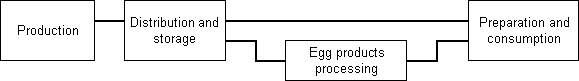
Production The production stage models the frequency of contaminated eggs at the time of lay and the level of bacteria initially present in contaminated eggs.

Distribution and storage The distribution and storage stage models growth in the number of Salmonella Enteritidis organisms between the laying of a contaminated egg and its preparation for consumption. Times and temperatures during storage and transportation can affect the microbe numbers within contaminated eggs.

Egg products processing The egg products stage models the occurrence and concentration of Salmonella Enteritidis in egg products.

Preparation and consumption The preparation and consumption stage models the effects of meal preparation and cooking on the number of Salmonella Enteritidis in meals containing egg. Eggs may travel different pathways depending on where they are used, how they are used, whether they are cooked, and to what extent they are cooked. Each of these pathways is associated with a frequency of occurrence and a variable number of servings. In addition, environmental conditions may differ for each pathway.

Previous exposure assessments

The drafting group identified five risk assessments previously conducted for Salmonella Enteritidis in eggs. They are briefly summarized below.

Salmonella Enteritidis and eggs: assessment of risk (Morris, 1990)

This simple analysis was conducted soon after the identification of the Salmonella Enteritidis epidemic in the United States of America. Data revealed that less than 1 in 1000 eggs from infected flocks were contaminated. An infected hen laid one contaminated egg in every 200, leading to an overall prevalence in endemic areas of 1 in 10 000 to 14 000 eggs produced. Approximately 0.9% of eggs were eaten without cooking. This report summarized Salmonella Enteritidis outbreaks and contributing risk factors for human infection. These risk factors included poor refrigeration practices, improper storage of pooled eggs, use of raw eggs, substantial time and temperature abuse of eggs, and exposure of highly susceptible individuals. The report also includes pertinent facts about Salmonella Enteritidis and eggs. Among the critical facts listed are that Salmonella Enteritidis has usual sensitivity to heat and is destroyed by pasteurization and cooking. Organisms may grow rapidly in egg mixtures (up to one log per hour), and warm summer temperatures may allow Salmonella Enteritidis to grow within shell eggs.

The analysis concluded by separating humans into four risk groups:

[1] Healthy adults who usually eat fully cooked eggs. The prevalence of contaminated eggs (i.e. 1 in 14 000) and the frequency of consuming raw eggs (0.9%) equated to a risk of one in 1.6 million eggs consumed. If an individual consumed 250 eggs per year and lived to 80 years old, the risk was reportedly one in 80 lifetimes.

[2] Healthy adults who frequently eat fried, soft boiled, and other less thoroughly cooked eggs. The risk for this group was not quantified, but thought to be higher than the first risk group.

[3] Healthy adults who eat eggs not fully cooked and frequently eat at restaurants and other places where pooling and abusive storage of eggs are possible. The risk for this group was thought to be proportional to the number of eggs pooled. If 10 eggs were pooled, the risk was 10 times greater. A specific quantification of risk for this group was not provided.

[4] More-susceptible individuals who eat higher-risk products as for group [3]. These individuals included residents of nursing homes and hospitals. No quantification of their risk was provided, but they are likely to be the population most at risk.

The assertions in Morris’ analysis are not supported by references to research or data, but the mechanics of the analysis should be transparent to most readers.

A farm-to-table exposure assessment should consider all possible scenarios where human illness results from Salmonella Enteritidis in eggs. However, Morris’ analysis was limited in the scenarios it considered and was, for the most part, non-quantitative. Therefore it was not considered in the comparative evaluation of different risk assessments for this report.

Risk assessment of use of cracked eggs in Canada (Todd, 1996)

The objective of this analysis was to determine the probability of illness associated with consuming cracked shell eggs in Canada. Eggs with cracks in the shell are considered hazardous because their contents are potentially exposed to pathogens more readily than eggs with intact shells. The hazard identification evaluated the possible association of Bacillus spp., Campylobacter spp., Salmonella, Staphylococcus aureus, Yersinia enterocolitica, Escherichia coli O157:H7 and Listeria monocytogenes with cracked eggs and human illnesses. Salmonella was the only hazard conclusively linked to human illness in this assessment. Therefore Salmonella was the only hazard used in further analysis.

Research was cited demonstrating that Salmonella can penetrate the shells of intact eggs. Nevertheless, it was concluded that little growth of Salmonella organisms would occur unless these organisms gained access to the yolk. Research was cited demonstrating that between 1.3% and 6.3% of eggs examined in Canada were cracked. Risk factors noted to be associated with processing included washing and rapid cooling. Both of these factors were thought to reduce shell integrity and make cracks more likely to occur. Research was cited demonstrating that Salmonella was more likely to be isolated from cracked eggs than from intact eggs.

The number of cracked shell eggs was estimated by multiplying the fraction of all eggs that were cracked by the number of eggs produced annually in Canada. To determine the illness burden, 13 outbreaks involving shell eggs were analysed and five of the outbreaks were identified as associated with cracked eggs. Given the estimated ratio of cracked to uncracked eggs, and the ratio of outbreaks associated with cracked eggs to those associated with intact eggs, a relative risk of 23:1 was calculated. Uncertainty analysis suggested the relative risk might range from 3:1 to 93:1.

By using reported human cases, adjusted for underreporting, Todd (1996) estimated that 10 500 cases per year are associated with cracked eggs. The risk of illness was calculated as one case per 3800 cracked eggs consumed, using an estimated exposure to 40 million cracked eggs.

This exposure assessment is transparent and data based. It relies on human epidemiological data to determine the illness burden associated with cracked eggs. Substantial uncertainty attends the estimates, but these are probably more defensible than a mechanistic farm-to-table model based on limited evidence. At the same time, assumptions regarding correspondence of eggs to cases are problematic, because a single egg may contribute to many servings. This effect is not captured by the analysis. Furthermore, the lack of a mechanistic explanation of the chain of events leading to illness makes risk management options difficult to evaluate. General policies, such as requiring all cracked eggs to be pasteurized, can be reasonably evaluated with this approach, but more subtle interventions, such as strict temperature-controlled storage requirements for cracked eggs, cannot be easily analysed without a mechanistic modelling approach.

Because this analysis was not a farm-to-table exposure assessment that incorporated quantitative data for each stage, it was not included in the comparative evaluation of exposure assessments. However, the approach used in this analysis is useful for certain types of exposure assessments that require rapid approximations of risk. In particular, preliminary assessments could be based on this approach to determine if a problem deems further, more time consuming, analysis.

Development of a quantitative risk assessment model for Salmonella Enteritidis in pasteurized liquid eggs (Whiting and Buchanan, 1997)

This farm-to-table quantitative risk assessment estimated the potential risks associated with consuming mayonnaise prepared from pasteurized liquid whole eggs. Although it does not consider all possible pathways that might lead to illness from pasteurized egg products, it comprises many of the components of a production-to-consumption exposure assessment. It was therefore included in this comparative evaluation of exposure assessments.

The exposure assessment model includes inputs on the proportion of commercial flocks that are affected by Salmonella Enteritidis (i.e. contain infected birds), the frequency that infected flocks produce contaminated eggs, the numbers of Salmonella Enteritidis in contaminated eggs, and the influence of time and temperature abuse on growth of Salmonella Enteritidis before and after pasteurization. This model also includes an input that predicts the effectiveness of pasteurization when applied according to regulatory standards. Time, temperature and pH inputs are varied to demonstrate their influence on the number of Salmonella Enteritidis organisms that remain in a serving of home-made mayonnaise prepared using pasteurized egg product.

This assessment determined that pasteurization reduced consumer risk associated with a high prevalence of Salmonella Enteritidis infection in layer flocks. Reducing time and temperature abuse of contaminated eggs before pasteurization was also effective for risk reduction. However, inadequate pasteurization temperatures and temperature abuse during post-pasteurization storage were associated with increased risk of human Salmonella Enteritidis exposure and illness.

Salmonella Enteritidis Risk Assessment: Shell Eggs and Egg Products (USDA-FSIS, 1998)

This farm-to-table quantitative risk assessment model examined the human illness risk associated with Salmonella Enteritidis in shell eggs, covering an exhaustive number of consumption pathways. It also examined the levels of Salmonella Enteritidis in liquid egg products before and after pasteurization. It contains the components of an exposure assessment from production to consumption, and is included here in the comparative evaluation of such analyses.

The exposure assessment model estimated the unmitigated risk of exposures resulting from consumption of table eggs that were internally contaminated with Salmonella Enteritidis. In concert with a hazard characterization, the baseline exposure assessment was then used to identify target areas for risk reduction activities along the farm-to-table continuum. These target areas could be further evaluated to compare the public health benefits accruing from the mitigated risk of Salmonella Enteritidis egg-borne illness resulting from various intervention strategies. Furthermore, the exposure assessment was used to identify data gaps and guide future research efforts.

Example mitigations included reduction of storage times and temperatures, reduction in the prevalence of infected flocks, and diversion of contaminated eggs. These were examined to evaluate the proportional effect on estimated human cases per year. Diversion of contaminated eggs resulted in a direct reduction in human cases, as did a mitigation strategy that combined reduction of the prevalence of infected flocks with reduction in egg storage times. Other mitigation scenarios were less efficient, but the costs of achieving any of the intervention strategies were not considered. A specific policy requiring storage of eggs at an ambient temperature at or below 45°F [7.2°C] before and during processing resulted in an average 8-12% reduction in human cases per year.

Salmonella Enteritidis in eggs risk assessment (Health Canada, 2000)

This farm-to-table quantitative risk assessment focused on Salmonella Enteritidis in table eggs. The FAO/WHO drafting group members for the present report were given a copy of the spreadsheet model for review and analysis. The model consists of all components of an exposure assessment, with the exception of egg products processing. It was therefore included in most of the comparative evaluation of exposure assessments.

The Whiting and Buchanan (1997), USDA-FSIS (1998) and Health Canada (2000) exposure assessments are discussed and the data quality and biases are evaluated. The pathways modelled in these exposure assessments are also compared. Discussions included the issues of variability and uncertainty - concepts important in the field of risk assessment. Variability describes naturally occurring observable differences within or between populations, while uncertainty describes our confidence about the true value of some parameter, or the frequency distribution of some variable; in essence, our understanding of the system under investigation. Uncertainty can be reduced by the gathering of more data, but variability cannot be changed without some intervention in the physical world. The explicit separation of variability and uncertainty for model inputs and outputs is a goal of risk assessors. Such separation allows decision-makers to understand how model outputs might improve if uncertainty were reduced. However, accomplishing this separation is a daunting task, so model inputs are described as uncertain, variable or both. Methods are also introduced for separating uncertainty and variability for inputs, as well as for model outputs.

Exposure assessments should be transparent to decision-makers. Through discussion and critical review, it is hoped that an understanding of the exposure assessments examined in this section will be attained.

4.2.2 Production

The production component of a Salmonella Enteritidis exposure assessment will produce an output consisting of a distribution of contaminated eggs at varying levels of contamination. This distribution describes the frequency of eggs that contain Salmonella Enteritidis bacteria per unit time or per egg. Additional outputs might describe the fraction of Salmonella Enteritidis contaminated eggs by geographic region, by flock type (e.g. battery or free range), or by other factors that distinguish egg production facilities (e.g. flock size).

Inputs to a production component include the prevalence of infected flocks; the frequency at which infected flocks produce contaminated eggs; the number of Salmonella Enteritidis bacteria initially present at the time of lay (or soon thereafter); and possibly moulting practices. These data may be derived from several sources, including prevalence studies of Salmonella Enteritidis in layer flocks, epidemiological studies of risk factors, transmission study results, industry demographic data, and experimental or survey data concerning the concentration of organisms in, or on, infected animals or their products.

Prevalence data are usually adjusted for the sensitivity or specificity, or both, of the diagnostic assay used. In this context, sensitivity describes the frequency that truly infected hens or flocks are detected using surveillance or testing protocols. Specificity describes the frequency that truly non-infected hens or flocks are properly classified as non-infected. Because diagnostic tests for the presence of Salmonella Enteritidis are based on microbiological culture, most analysts assume that specificity is 100%. Surveys typically use diagnostic tests with imperfect sensitivity and do not sample all birds in the flock. Imperfect laboratory tests result in biased estimates of the number of infected hens in flocks. Sampling less than 100% of the birds in a flock can result in misclassification of infected flocks.

The availability of detailed epidemiological data provides better risk assessments. Increased detail provides information that is more precise for decision-making based on risk assessments. For example, the proportion of all eggs in a country or region that are contaminated can be calculated from: (1) an estimate of the proportion of flocks containing Salmonella Enteritidis-infected hens, and (2) the proportion of eggs laid by these flocks and which are contaminated. An estimate of the contaminated egg proportion could be derived from a random sampling across all egg production, but such an approach is extremely costly and not useful for analysis of mitigation of the risk to humans when the estimate is unattached to status of the producing flock. For example, if a random sample of eggs across the country estimated that 1 egg in 20 000 was contaminated, this information may be of little value to decision-makers without information about spatial and temporal clustering of infected flocks. One could not determine whether some flocks produce contaminated eggs more frequently than others (i.e. spatial clustering), nor could one determine if there were certain times when flocks produce more contaminated eggs (i.e. temporal clustering).

Many factors contribute to variability in the production of contaminated eggs. These include regional differences in flock prevalence - if egg marketing is regional - and flock age. Other factors (e.g. stage of infection in flock, season, control efforts by management) may also modulate within-flock prevalence and egg contamination frequency. Moult status of flocks is a proven risk factor that can influence flock-to-flock variability in egg production and egg contamination frequency.

Flock prevalence

By definition, flock prevalence is the proportion of flocks containing one or more birds infected with Salmonella Enteritidis. As contaminated eggs can only be produced by infected flocks, exposure assessments must concentrate on these flocks.

Flock prevalence data always represents apparent prevalence. Apparent prevalence is the observed prevalence without accounting for the effects of diagnostic test imperfections. For present purposes, apparent prevalence equals the true prevalence of infection times the sensitivity of the methods used to generate the observations.

Most evidence suggests that infected flocks remain infected for most of their productive life. Hens usually begin egg production at about 20 weeks of age. Flocks usually become infected soon after immature hens (i.e. pullets) are placed in laying houses. Carryover infection from a previously infected flock and rodent reservoirs in the environment of such flocks serve to perpetuate infection across flocks. Infection of flocks during pullet grow-out probably can occur via a previously contaminated environment. Infection at the hatchery is also possible.

Local trends in flock prevalence for a country or region might be inferred from surveillance data. Such an inference might suggest that the proportion of infected flocks in a country or region is increasing or decreasing over time. Nevertheless, these trends must be demonstrated across a sufficient period to be convincing. Cross-sectional surveys may imply seasonal patterns in flock prevalence, but this is not likely to be the case. Instead, observed seasonal differences in flock prevalence in cross-sectional studies are probably the result of changes in within-flock prevalence and the effect of increases or decreases in within-flock prevalence on the capacity of a survey to detect infected flocks. Therefore, unless local trends are clearly proven, it is generally best to model flock prevalence as an invariant, fixed value. The methods used to model flock prevalence should incorporate all uncertainty regarding the true fixed value.

Data

Table 4.1 summarizes data on flock prevalence. The three quantitative exposure assessments have used some of these data to estimate flock prevalence.

Table 4.1. Studies to determine the proportion of layer flocks that contain one or more infected hens.

The studies in Table 4.1 differ in the number of flocks sampled, the intensity of sampling within each flock and the test methodology, as well as in the reported apparent prevalence. Because flock prevalence is constant, the main interest becomes describing the uncertainty about the true value, so methods are described for modelling this uncertainty. Furthermore, apparent prevalence estimates are biased, so methods are described to correct this bias.

Methods

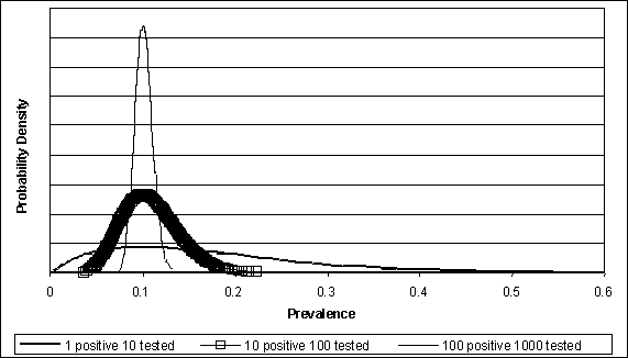
The Beta distribution is commonly used to model prevalence in quantitative exposure assessments. When using the @Risk^® software (Palisade Corporation, Newfield, NY), this distribution is modelled as @RISKBETA(s+1,n-s+1), where s is the number of positives observed and n is the total number sampled. This distribution can be derived by applying Bayes Theorem to the binomial distribution, where p is the probability of a positive, or prevalence (Vose, 1996). The Beta distribution demonstrates the increased certainty in estimated prevalence resulting from increasing the number of samples collected. For example, Figure 4.2 illustrates how a probability density function becomes increasingly narrowed for increasing numbers of samples when the underlying prevalence of positives is fixed at 10%.

Figure 4.2. Illustrating the effect of increased sample size on certainty regarding prevalence.

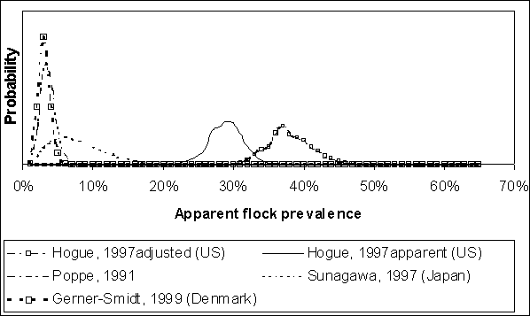
Data similar to those presented in Table 4.1 are typically used to estimate regional or national flock prevalence. In the US SE RA, the data from Hogue et al. (1997) were used to estimate the United States of America flock prevalence. These data were generated from sampling hens at slaughter plants, and summarized at a regional level (Figure 4.3).

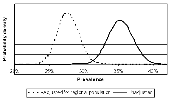
The proportion of all flocks sampled in these four regions did not match the proportion of regional production. Instead, more flocks were sampled in the high prevalence regions. Therefore the raw data were adjusted by calculating the expected value of prevalence:

where p_i was the observed prevalence in region i, and w_i was the proportion of production in region i. The total number of positive flocks was calculated as the product of this expected value and the observed number in Table 4.1. The total number of flocks sampled (i.e. 711) was not changed, so the uncertainty in the estimated prevalence was consistent with the level of sampling used. Figure 4.4 shows the effect of this adjustment on apparent flock prevalence.

Given apparent prevalence evidence like that shown in Table 4.1, exposure assessment models must make adjustments for false-negative results. No survey of flocks can definitively determine the status of flocks sampled. Given the limited number of flocks sampled in surveys, the limited sampling within flocks, and the imperfect nature of diagnostic tests applied to individuals - and our imperfect understanding of these imperfections - uncertainty about true flock prevalence can be substantial.

Figure 4.3. Regional results of USA spent hen surveys (Hogue et al., 1997) and percent of USA flocks by region. National estimates of flock prevalence should be adjusted for spatial bias.

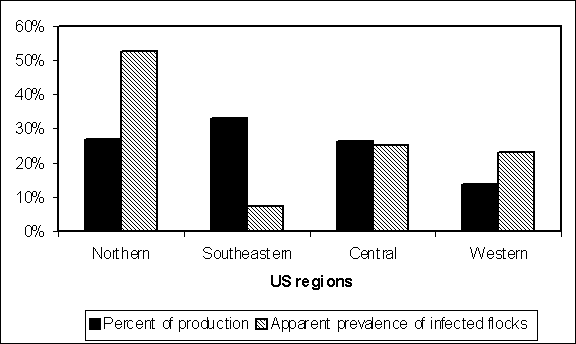
Figure 4.4. Illustration of the effect of weighting USA survey results (Hogue et al., 1997) for regional hen populations to estimate uncertainty regarding the national flock prevalence

Two factors influence the likelihood of false-negative results: the number of hens sampled per flock, and the underlying likelihood of detecting an infected hen given the methods used to test individuals.

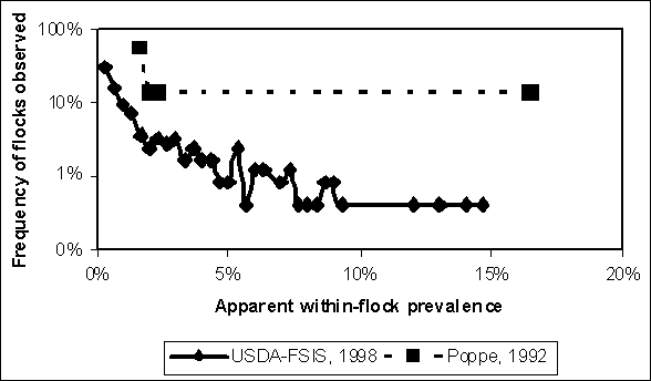
Tables 4.2 and 4.3 show the results of sampling within infected flocks. The Poppe et al. (1992) study was a follow-up to the survey listed in Table 4.1. The original survey identified eight infected Canadian flocks, but was able to measure within-flock prevalence in only seven flocks. A variable number of hens were cultured in each of these flocks and, in four flocks, no infected hens were detected, despite previous positive hen or environmental test results, or both. The mean of the Beta distribution based on these results provided a non-zero point estimate for within-flock prevalence (Table 4.2). Table 4.3 summarizes the findings of the studies analysed by Hogue et al. (1997). In two different surveys, 247 positive flocks were detected. For each flock, 60 pooled caecal samples comprising five hens each were collected (i.e. caecae were collected from 300 hens per flock). Apparent within-flock prevalence was estimated by assuming that only one infected hen contributed to each positive pool. Such an assumption is reasonably unbiased (i.e. <5% difference between assumed and calculated within-flock prevalence) for those flocks with up to seven positive pools, but this negative bias increases with the number of positive pools. The average bias from this simplifying assumption is 5% across all observations.

Tables 4.2 and 4.3 provide evidence of the variability in number of S. Enteritidis infected hens between infected flocks. Both studies suggest that low within-flock prevalence is more frequent than high within-flock prevalence (Figure 4.5). Despite different populations sampled (e.g. Canadian vs United States of America layer flocks) and the dramatically different numbers of samples collected, the distributions are similar.

Table 4.2. Results of sampling known-infected layer flocks from Canadian study and mean of Beta distribution for predicting apparent within-flock prevalence

SOURCE: Poppe et al., 1992

Table 4.3. Results of sampling known-infected layer flocks from USA studies. To calculate within-flock prevalence, it is assumed that a positive pool is equivalent to one positive hen, and 300 hens (60 pools of 5 hens) were sampled per flock.

SOURCE: Hogue et al., 1997

Figure 4.5. Comparison of evidence for within-flock prevalence from two studies that sampled multiple infected flocks.

Flock prevalence estimation methods have been proposed (Audige and Beckett, 1999; USDA-FSIS, 1998). These methods account for less-than-complete sampling within flocks. Given a fixed within-flock prevalence, infected flocks can be incorrectly classified as negative when a limited number of samples are collected in the flock (Martin, Meek and Willeberg, 1987). In practice, sample size is usually fixed in surveys, while within-flock prevalence varies between infected flocks. Therefore, collecting a number of samples sufficient to detect at least one positive hen in one infected flock (with reasonable likelihood) may not be a sufficient number in another infected flock.

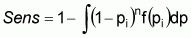
In the US SE RA, the probability that a positive flock is detected given a fixed sample size is calculated as 1-(1-p)ⁿ, where p is apparent within-flock prevalence (i.e. proportion of detectable infected hens within an infected flock) and n equals the number of hens sampled per flock. Apparent within-flock prevalence was modelled as a cumulative distribution based on the survey evidence in Table 4.3. The cumulative distribution (Vose, 1996) converts within-flock prevalence data into a continuous probability function by specifying the minimum possible value (arbitrarily set at 0.001%, or 1 in 100 000 hens), the maximum value (arbitrarily set at 100% of hens), and the evidence in Table 4.3. Integrating 1-(1-p)ⁿ across the distribution for apparent within-flock prevalence indicated that the sample size of 300 hens per flock used in the Hogue et al. (1997) surveys detected 76% of infected flocks. Integration was accomplished by simulating 1-(1-p)ⁿ, where p varied from iteration to iteration, and calculating the average of the simulated output.

For the US SE RA, the number of truly infected flocks in the Hogue et al. (1997) surveys was modelled using a Negative Binomial distribution. In the @Risk software language, the @RISKNEGBIN(s,p) function predicts the number of flocks missed given the number successfully detected, s, and the probability, p = 0.76, of detecting flocks (Vose, 1996). Adding the number of infected flocks misclassified in the survey to the number of infected flocks actually observed, then using this estimate with the total number of flocks sampled (i.e. 711) as inputs to a Beta distribution, provides the best description of uncertainty regarding true national prevalence.

An alternative to the method described for the US SE RA is to use a direct Bayesian methodology. In this case, Bayes Theorem is used to estimate the true flock prevalence:

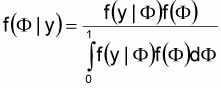
This depiction of Bayes Theorem is used to predict the distribution for flock prevalence (F), given the available evidence (y) (i.e. f(F|y)). In this case, the likelihood function, f(y|F), calculates the likelihood of observing a particular sampling result (e.g. 247 positive flocks in 711 flocks sampled) given that the true flock prevalence is F.

The likelihood function, f(y|F), determines the probability of the sampling evidence (i.e. apparent flock prevalence), given the true prevalence, F, and the sensitivity of the survey design. In this case,

where p_i is the apparent within-flock prevalence in flock i, f(p_i) is the likelihood of p_i occurring, and n is the number of samples collected in each flock. Operationally, the likelihood function is the binomial distribution,

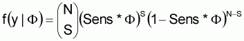
where N is the number of flocks sampled in a study, and S is the number found positive. Although this approach was not used in the US SE RA, it should give similar results to the negative binomial method previously described.

The Health Canada (2000) and Whiting and Buchanan (1997) exposure assessments did not adjust flock prevalence evidence for sensitivity. In the Health Canada assessment, the Poppe et al. (1991) data were modelled directly using a Beta distribution. In the Whiting and Buchanan (1997) assessment, two fixed values were used to model flock prevalence: 10% and 45%. These values were selected to approximate the regional variability observed in the United States of America surveys of slaughtered hens (Hogue et al., 1997).

Simply modelling apparent flock prevalence will result in a depiction of this parameter that differs from that found if true flock prevalence is modelled. Figure 4.6 illustrates the Beta distributions implied by the data in Table 4.1. In the case of the Hogue et al. (1997) data, the distribution that results from estimating true prevalence from apparent prevalence is illustrated. The effect of this adjustment is to shift the distribution towards higher flock prevalence levels, as well as slightly increasing the spread of the distribution.

Figure 4.6. Implied distributions for apparent flock prevalence using the sampling evidence listed in Table 4.1. Evidence was modelled using Beta distributions. The Hogue et al. (1997) data are modelled for both apparent prevalence (using just the sampling evidence), and after adjusting the sampling evidence for false-negative flocks (i.e. true prevalence).

Egg contamination frequency

Ideally, egg-culture data would be available from flocks known to be infected. However, results from sampling eggs from infected flocks will show variability across time in the same flock, and between flocks. Variability is expected in any biological system. Seasonal variability in egg culturing results may also be observed, but previous analysis has not detected a consistent pattern (Schlosser et al., 1999).

Unfortunately, the logistics and cost of egg sampling limit the availability of such data. Furthermore, when egg sampling is conducted at the flock level, the number of eggs sampled is usually inadequate to calculate precise estimates of egg contamination frequency. In fact, the low apparent prevalence of contaminated eggs from infected flocks suggests that inadequate sampling of eggs will usually result in culture-negative results for all samples collected.

Sampling eggs is not a cost-effective surveillance method when the prevalence of egg contamination in infected flocks is low (Morales and McDowell, 1999). It is possible, however, that variability in egg contamination from flock to flock might be modelled using evidence concerning within-flock prevalence of infected hens. Evidence may come from the proportion of hens in a flock that are faecal shedders of Salmonella Enteritidis, or have organ or tissue samples that are culture-positive for Salmonella Enteritidis. Regardless of the endpoint measured, some estimate of the fraction of contaminated eggs laid by infected (or colonized) hens will allow the modelling of egg contamination frequency at the flock level. However, uncertainty regarding the variability in egg contamination frequency is greater using this approach than one that relies on direct egg culturing evidence. For that reason, this approach to estimating egg contamination frequency is not preferred when direct egg culturing evidence is available.

Data

Tables 4.4 and 4.5 summarized the egg sampling evidence from known infected flocks or hens used by the three quantitative exposure assessments. These data are used in the respective models to estimate egg contamination frequency.

For the US SE RA and Health Canada exposure assessments, two forms of data from the same field project are used. The Health Canada exposure assessment data are from a study of 43 positive flocks; the number of samples analysed was limited to the first 4000 eggs collected from these flocks. In contrast, the complete egg sampling results from the 43 flocks were summarized in the US SE RA. The flocks were stratified into high and low prevalence in the US SE RA analysis. The basis of this stratification was the finding that egg contamination frequency was correlated with environmental status and there was a bimodal pattern to environmental test results in infected flocks. Additional studies were included in each strata, based on the same criteria or similarity in results. The combined results from the US SE RA study suggest an overall egg contamination frequency of 0.03%; the same as the average based on the Health Canada exposure assessment data.

In the Whiting and Buchanan (1997) model, the egg contamination frequencies implied by 27 published studies were summarized (Table 4.5). Some of these studies were reportedly experimental. The relevance of experimental studies to populations of naturally infected hens is arguable. In particular, if a study reports the frequency at which a cohort of experimentally inoculated hens produced contaminated eggs, then these results need adjusting for the prevalence of naturally infected hens in a flock to be comparable to field-based evidence. The median frequency from this series of studies is between 0.6% and 0.9%.

Table 4.4. Summary of evidence used in two exposure assessments to model egg contamination frequency. The number positive eggs (s) and the total number of eggs sampled (n) are reported by study cited

Table 4.5. Summary of evidence used to model egg contamination frequency in the Whiting and Buchanan (1997) exposure assessment model

Methods

A histogram relating egg contamination frequency with the number of infected flocks observed can be derived if enough eggs from enough flocks are sampled in a cross-sectional survey. Such a histogram provides an empirical description of the variability in egg contamination. This distribution may be skewed if most flocks express very low egg contamination frequencies and few flocks experience higher contamination frequencies.

In surveys that are prospective and cross-sectional in design, the data can be summarized using the average contamination frequency across all egg collections in each flock. Because individual egg collections usually involve an insufficient numbers of eggs (e.g. 1000), the most confident estimate is that applied to the entire period during which sampling was completed in that flock.

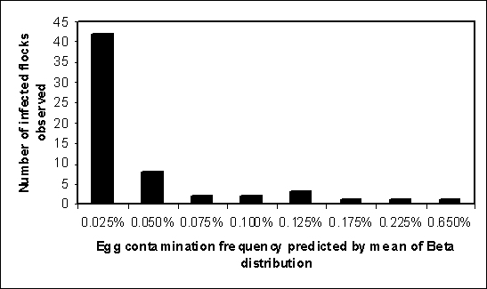
Figure 4.7 illustrates the distribution for egg contamination frequency found in one research project covering 60 infected flocks (Henzler, Kradel and Sischo, 1998). The reported frequencies are set equal to the mean of the Beta distribution to provide non-zero estimates for those flocks where no positive eggs were detected. A significant finding from this study was that a high proportion of the flocks with the lowest observed egg contamination frequency were also flocks with fewer numbers of positive environmental samples. Most of the flocks with higher egg contamination frequencies also had more positive environmental samples.

Egg contamination frequency evidence should be adjusted for uncertainty resulting from pooling of samples, and the sensitivity or specificity, or both, of laboratory culture techniques (Cowling, Gardner and Johnson, 1999). For pooled sample results, it is probably appropriate, when prevalence is low (e.g. <0.1%), to assume that individual prevalence is equivalent to x/km, where x is the number of positive pools, k is the size of pools (e.g. 10 or 20 eggs), and m is the number of pools sampled. Nevertheless, it is instructive to evaluate the probability theory of pooling.

Given some probability that an individual egg is positive, p, and a pool size of k, the probability of a pool being positive, P, equals 1 -(1 - p)^k, where (1 - p)^k calculates the probability of selecting k negative individuals. From available sampling evidence, we have P. Therefore we can solve this equation for p, and it equals 1 -(1 - P)^1/k. Cowling, Gardner and Johnson (1999) present various methods for describing the uncertainty about this estimated probability. A simple method is to describe the uncertainty about P as a Beta(x + 1, m - x + 1) distribution and directly map the values for p to the probabilities predicted for the Beta distribution. When p is very small and m is very large, the need to incorporate uncertainty about the effect of pooling is insubstantial.

Figure 4.7. Results of a study in 60 United States of America infected flocks, showing variability in egg contamination frequency between infected flocks (Source: Henzler, Kradel and Sischo, 1998).

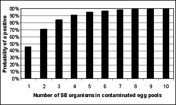
Evidence for the sensitivity of laboratory culture techniques comes from an experiment on the isolation of Salmonella Enteritidis in pooled eggs. In this study, pools of 10 eggs were spiked with approximately 2 CFU of Salmonella Enteritidis, and 24 out of 34 (70.6%) of the pools were detected as positive using standard culture techniques (Gast, 1993). Although Cowling, Gardner and Johnson (1999) argue that the best estimate of sensitivity for pooled egg culturing should be centred about 70.6%, this estimate may understate the likelihood of detection. Most contaminated eggs, unless cultured within a few hours of lay, contain many more than two Salmonella Enteritidis organisms (see section below). Therefore one must calculate the probability that laboratory culturing will detect a single organism and then apply that probability to the number of organisms expected to be found in contaminated egg pools.

If a pooled sample contains two Salmonella Enteritidis organisms, the probability of correctly classifying the sample as positive using culture techniques equals 1 -(1 - p)², assuming a binomial process and p equal to the probability of detecting one organism. From Gast (1993), 70.6% of samples with two Salmonella Enteritidis organisms were found positive. Therefore one can solve for p to determine the probability of detecting one organism in a pooled sample. In this case, p equals 46%.

If the probability of detecting one organism in a pooled sample is 46% - and the probability of detecting two organisms is 70.6% - then one can calculate the sensitivity of pooled egg testing for any number of organisms contained in a sample. Figure 4.8 shows how the probability of a positive result increases as the number of organisms in the sample increases. At eight organisms (or more) in a pooled sample, the probability of a positive test result is essentially 100%. Given that the predicted mean number of Salmonella Enteritidis organisms per contaminated egg typically exceeds seven, these results suggest it is unlikely that sensitivity of egg testing is an important input to exposure assessments.

Figure 4.8. Predicted probability of a positive pooled egg sample when contaminated with varying numbers of Salmonella Enteritidis (SE) organisms and a probability of detecting just one organism equal to 46%.

The frequency that an infected flock produces contaminated eggs is modelled in the Health Canada exposure assessment by incorporating the data in Table 4.4 into a gamma distribution. In @Risk, this distribution is specified as: @RISKGAMMA(s,1/n), where s is the number of positive eggs and n is the total number of eggs sampled. The gamma distribution is a theoretical distribution for estimating uncertainty about the average of a Poisson process. In practice, the difference is insignificant between assuming egg contamination frequency follows either a binomial or a Poisson process. Therefore, either the gamma or the beta distribution would suffice for modelling these data.

One can model the data cited for the Whiting and Buchanan (1997) exposure assessment (Table 4.5) using a cumulative distribution. In @Risk, the cumulative distribution is specified as:

@RISKCUMULATIVE(min,max, {x}, {p})

where theoretical minima and maxima are estimated, {x} is an array of observed egg contamination frequencies, and {p} is an array of cumulative probability densities corresponding to values in {x}. Alternatively, these data could be modelled using discrete or histogram distributions.

In the US SE RA exposure assessment, egg contamination frequencies for high and low prevalence flocks are modelled using the gamma distribution. The egg contamination frequencies for each type of infected flock only apply to the fraction of infected flocks within these two strata. This exposure assessment also explicitly models moulted and non-moulted flocks. Therefore, egg contamination frequency from infected flocks is calculated as a weighted average across all infected flocks by prevalence strata and moult status.

The data in Table 4.5 on the frequency of Salmonella Enteritidis-positive eggs produced by positive flocks were from flocks that were typically detected via environmental sampling. Estimating egg contamination frequencies directly from these data can result in biased estimates, possibly introduced because environmental testing is more likely to detect infected flocks with high within-flock prevalence levels, compared with flocks with low within-flock prevalence levels. Therefore, egg-culturing evidence is disproportionately influenced by higher prevalence flocks relative to the actual egg contamination frequency in the total population of infected flocks. In US SE RA, the proportion of infected flocks classed as high prevalence was adjusted for the sensitivity of environmental testing to account for this phenomenon.

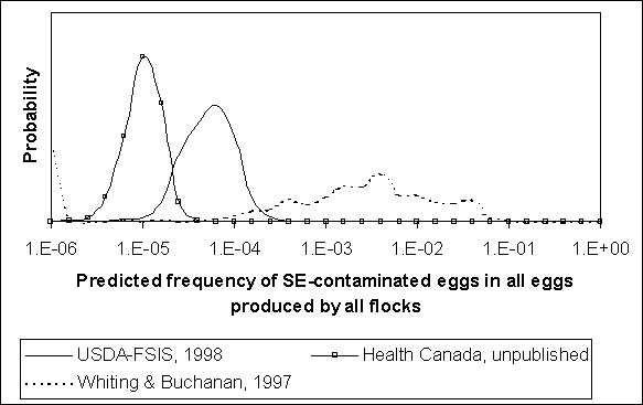
The effect of moulting on egg contamination frequency has been experimentally examined and found significant (Holt and Porter, 1992, 1993; Holt et al.,1994; Holt,1995, 1998). However, there is only one field study that examines this phenomenon (Schlosser et al., 1999). In that study, 31 of 74 000 (0.04%) eggs sampled from infected flocks that were within 20 weeks following moult were Salmonella Enteritidis-positive. In contrast, only 14 of 67 000 (0.02%) eggs sampled from infected flocks that were within 20 weeks prior to moult were Salmonella Enteritidis-positive. These results imply that moulting is associated with a nearly twofold increase in egg contamination in the 20 weeks following moult. Figure 4.9 shows the probability distributions for high and low prevalence flocks that are moulted or not moulted, using these data and those shown in Table 4.4. Figure 4.10 illustrates the different distributions for egg contamination frequency in infected flocks, generated by the three exposure assessments. The weighting of egg contamination frequencies for different types of flocks in the US SE RA has the effect of reducing the overall frequency of contaminated eggs from infected flocks. Nevertheless, the predicted distributions for the US SE RA and Health Canada exposure assessments are more similar to each other than either is to the distribution implied by Whiting and Buchanan (1997). The Whiting and Buchanan (1997) distribution is bimodal, with some flocks producing contaminated eggs at frequencies at or below 10^-6 and many more flocks producing contaminated eggs at frequencies at or above 1%.

It should be noted that the US SE RA and Health Canada distributions in Figure 4.10 represent uncertainty about the true fraction of contaminated eggs produced by infected flocks. In contrast, the Whiting and Buchanan (1997) distribution is best characterized as a frequency distribution of the predicted proportion of infected flocks producing contaminated eggs at different frequencies. Only the reported frequencies, and not the number of positives and samples, were used to derive this distribution. Therefore uncertainty about the true egg contamination frequencies reported by each of the 27 studies used by Whiting and Buchanan (1997) is not incorporated into this analysis.

Figure 4.9. Comparison of uncertainty regarding egg contamination frequencies between so-called high and low prevalence flocks that are moulted or not moulted (Source: US SE RA).

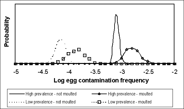
Figure 4.10. Uncertainty regarding egg contamination frequency in infected flocks as predicted by three published exposure assessments.

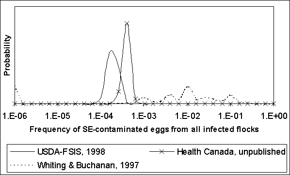
The proportion of flocks that are infected (i.e. flock prevalence) and the egg contamination frequency for infected flocks are combined to estimate the overall frequency of contaminated eggs among all eggs produced. Figure 4.11 shows these results for the three quantitative exposure assessments. For both the US SE RA and Health Canada exposure assessments, the predicted fraction of all eggs that are Salmonella Enteritidis-contaminated is most probably between 10^-5 and 10^-4. The overall contamination frequency implied by Whiting and Buchanan (1997) is most probably between 10^-3 and 10^-2.

Figure 4.11. Uncertainty regarding frequency egg contamination by Salmonella Enteritidis (SE) among all eggs produced, regardless of flock status, as predicted by three published exposure assessments.

Methods for modelling egg contamination frequency varied among the three quantitative exposure assessments. Although the USDA-FSIS and Health Canada approaches are similar in some respects, the US SE RA explicitly modelled variability in egg contamination frequency by stratifying infected flocks into different categories (e.g. high and low prevalence). Disaggregation of infected flocks by degree of severity accomplishes two purposes: first, it allows one to explicitly model control interventions on a subset of the total population of infected flocks; and, second, it illustrates the relative importance of different types of flocks to the overall frequency of contaminated eggs. By modelling high and low prevalence flocks, as well as moulted or unmoulted subpopulations, the US SE RA may be a more useful tool for risk managers. Furthermore, the explicit delineation of flocks because of severity of their infection enabled the identification of a potential bias resulting from easier detection of the more severely affected flocks.

The methods used by Whiting and Buchanan (1997) may illustrate the possible bias introduced using experimental data. Egg contamination frequency in infected flocks is best estimated using field research results. Experimental studies cannot replicate the infectious dose and transmission characteristics that exist in naturally infected flocks. This distribution may also imply increased egg contamination frequencies because the underlying data reflect higher-virulence strains of Salmonella Enteritidis than typically occur in naturally infected populations (Gast, 1994).

Ideally, this exposure assessment input should describe the variability of egg contamination frequency between infected flocks. Although the US SE RA accomplishes this to a limited extent by stratifying flocks, a more continuous description of this input is desirable. Either the gamma or the beta distribution can be used to model uncertainty in egg contamination frequency based on the available data. Furthermore, given the numbers of organisms expected within contaminated eggs, and the low frequency of contaminated eggs, it seems unnecessary to adjust observed data for pool size or sensitivity of tests.

Organisms per egg at Lay

An exposure assessment must include the initial concentration of Salmonella Enteritidis in contaminated eggs. The number of S. Enteritidis in contaminated eggs varies from egg to egg. Available evidence suggests that most contaminated eggs have very few S. Enteritidis bacteria within them at the time of lay. It is the initial contamination level in an egg that is influenced by subsequent distribution and storage practices. If the egg is handled under conditions that allow growth of the bacteria in the egg, then the initial concentration will increase. Nevertheless, some contaminated eggs will arrive at the kitchen with the same number of bacteria within them that they contained at the time of lay.

Most experts believe the S. Enteritidis in eggs is initially limited to the albumen or vitelline (yolk) membrane. Nevertheless, it is possible that S. Enteritidis may gain access to the yolk of the egg before or just after the egg is formed. If this occurs, it is a rare event. While egg albumen is not conducive to S. Enteritidis multiplication, yolk nutrients will foster relatively rapid growth of these bacteria (Todd, 1996).

Immediately following lay, the pH of the interior contents of an egg begins to increase. Elevated pH suppresses growth of S. Enteritidis. It is estimated that about one log of growth can occur between the time of lay and stabilization of pH inside the egg (Humphrey, 1993). Because of this phenomenon, it is difficult to know whether the observed number of organisms in a fresh egg is the result of some initial growth or the actual inoculum present at lay.

Data

In a study of contaminated eggs produced by naturally infected hens, 32 positive eggs were detected (Humphrey et al., 1991). Enumeration of their contents found that 72% of these eggs contained less than 20 S. Enteritidis organisms. The calculated mean number of S. Enteritidis per contaminated egg was 7. However, there were a few eggs that contained many thousands of S. Enteritidis bacteria following >21 days of storage at room temperature.

In a study of experimentally infected hens, 31 Salmonella Enteritidis positive eggs were detected (Gast and Beard, 1992a). Enumeration of their contents found that the typical contaminated egg harboured about 220 Salmonella Enteritidis organisms. Yet, there were marked differences in levels depending on storage time and temperature. Four of the contaminated eggs contained more than 400 Salmonella Enteritidis organisms per egg.

Methods

Growth of bacteria within the egg is a function of temperature and time between lay and consumption. At the time of lay, the egg’s internal temperature is essentially that of the hen (i.e.~42°C). This temperature equilibrates with the environment over time.

Conventionally, concentration of bacteria per unit volume is modelled using a lognormal distribution (Kilsby and Pugh, 1981). Such a distribution describes the frequency of variable numbers of bacteria in contaminated eggs. Assuming there is sufficient data to estimate a population distribution, then uncertainty in an exposure assessment model stems from the fitting procedure used to describe the distribution. Lacking evidence from a sufficient sample of eggs to warrant direct fitting of evidence to a distribution, alternative approaches include using expert opinion to develop a distribution, or representing the data with an empirical distribution.

In the Whiting and Buchanan (1997) exposure assessment, a two-stage distribution for concentration of organisms per contaminated egg is modelled. The majority of eggs are modelled as containing 0.5 organisms/ml. For a 60-ml volume egg, this equates to 30 organisms per egg. Development of this estimate is based on the Humphrey et al. (1991) enumeration data. Some eggs in the Whiting and Buchanan (1997) model, however, are assumed to be held for up to 21 days at room temperature, or for shorter times at higher temperatures. These eggs experience growth of S. Enteritidis and the resultant number of organisms per egg is modelled using the following probability distribution: 58% = 0.5 organisms/ml; 25% = 13 organisms/ml; 8% = 375 organisms/ml; and 8% = 3 000 organisms/ml. Because this model is concerned with eggs that are sent for pasteurization, the large concentrations predicted here are arguably appropriate.

The fraction of eggs that are time- or temperature-abused in the Whiting and Buchanan (1997) model is assumed to range from 2.5% to 10% of all eggs. Therefore contaminated eggs usually contain about 30 organisms, but for 2.5-10% of this model’s iterations the eggs may contain from 30 to 180 000 organisms.

In the Health Canada exposure assessment, data from two studies are combined to depict initial concentration. An initial number of organisms is modelled as the output of a Poisson process, where the mean is 7 organisms per egg (Humphrey et al., 1991). To this initial number of organisms is added another 0 to 1.5 logs of bacteria to account for the period immediately after lay, when pH is increasing in the egg (Humphrey, 1993; Humphrey and Whitehead, 1993). This additional step is modelled using the @Risk function @RISKPERT(min, most likely, maximum),where the minimum is zero, the most likely value is 1 log, and the maximum is 1.5 logs.

In the US SE RA, the data from Humphrey et al. (1991), Humphrey (1993) and Gast and Beard (1992) are combined to derive a distribution for initial number of S. Enteritidis organisms per contaminated egg. A truncated exponential distribution is used to model this input. In @Risk, this distribution is specified as @RISKTEXPON(mean, min, max), where the minimum equals 1 organism, the maximum is 420 organisms (based on Gast and Beard, 1992), and the mean is 152 organisms per egg.

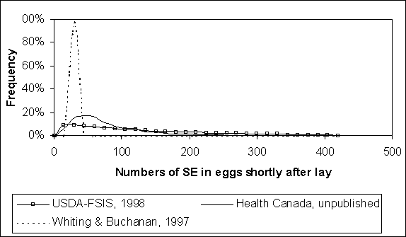
The effect of the different modelling approaches used in the three exposure assessments is shown in Figure 4.12. The curve predicted by Whiting and Buchanan (1997) shows a peak frequency at 30 organisms per egg; however, the instances of heavily contaminated eggs are not shown in this graph. Although heavily contaminated eggs are infrequently predicted, the expected value of this distribution (>900 organisms per egg) reflects these occasionally large values.

The expected values of the Health Canada and US SE RA distributions are 88 and 152 cells, respectively. The US SE RA distribution reflects the incorporation of the Gast and Beard (1992) evidence. This evidence is from experimentally infected hens that were inoculated with large doses of S. Enteritidis. Its relevance to naturally contaminated eggs is arguable. Nevertheless, the combined evidence from Humphrey et al. (1991) and Gast and Beard (1992) amounts to just 63 eggs. Therefore the USDA-FSIS distribution may be interpreted as containing elements of variability and uncertainty regarding the actual frequency distribution for initial contamination levels in eggs.

Figure 4.12. Comparison of varying levels of Salmonella Enteritidis (SE) within contaminated eggs, predicted by three published exposure assessments

Summary

The production component of an exposure assessment should include estimates of flock prevalence, egg contamination frequency in infected flocks, and number of S. Enteritidis per contaminated egg.

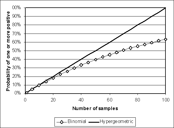
Flock prevalence is arguably a fixed value, but one for which uncertainty can be substantial. Apparent flock prevalence from surveys that use imperfect diagnostic assays should be adjusted for expected bias. Several methods are available to make these adjustments. Audige and Beckett (1999) have published a method that relies on the hypergeometric distribution. Such a method is particularly appropriate when the total population is small. The consequence of incorrectly assuming evidence was generated from a binomial distribution (that assumes sampling with replacement in a large population) is illustrated in Figure 4.13.

This example assumes that just one infected flock exists in a total population of 100 flocks. The probability of detection in this case is different if we assume a binomial distribution versus assuming the correct hypergeometric distribution. If we had a sample of 100 flocks and all were negative, the binomial distribution would imply that there was a 40% chance of such a result if the prevalence was 1%. In contrast, the hypergeometric distribution would tell us there was 0% probability of such a result if one infected flock existed. The probability of detection is used to adjust apparent flock prevalence, so it behoves the risk analyst to consider which distribution is appropriate when conducting an exposure assessment.

Figure 4.13. Illustration of the effect of assuming a binomial distribution when the population is limited to 100 and the prevalence is fixed at one infected flock (1%)

None of the exposure assessments explicitly accounted for the mechanisms by which flocks become infected. To assess pre-harvest interventions, more data is needed on the prevalence of S. Enteritidis in breeder and pullet flocks, as well as in feedstuffs. In particular, associations between the occurrence of S. Enteritidis in these pre-harvest steps and its occurrence in commercial layers should be quantified. The existing models, however, can be used to evaluate the effect of interventions that might reduce the risk of flocks becoming infected. The public health effect of such hypothetical interventions would be modelled by appropriately reducing the flock prevalence input of the existing models.

Egg contamination frequency should be a variable input to a S. Enteritidis exposure assessment. However, data are needed to accurately estimate the proportion of flocks with varying egg contamination frequencies. An alternative to modelling egg contamination frequency as a continuous distribution is to stratify flocks into two or more categories and model the estimated egg contamination frequency separately for each category. Such an approach provides more information to risk managers regarding control options. Nevertheless, stratifying infected flocks requires epidemiological evidence of differences among infected flocks. Without such evidence, use of available egg sampling evidence is a second-best approach.

The concentration of S. Enteritidis in contaminated eggs is also a variable input, yet few data are available to describe this variability. In the exposure assessments evaluated, estimation of the number of S. Enteritidis in contaminated eggs at, or soon after lay, was based on empirical data from, at most, 63 eggs. Evidence that associates modulation in numbers of S. Enteritidis per egg with causative factors (i.e. strain of S. Enteritidis, hen strain, environmental conditions) would provide analysts with better methods for modelling this input. Lacking such evidence, however, suggests that most S. Enteritidis exposure assessments will rely on the same evidence used by previous exposure assessments. Therefore, it is expected that this input will be common to most models. Of the methods used to model initial contamination, those used by Health Canada seem most intuitively appealing. The method used by US SE RA gives similar results but is potentially biased upwards.