5. TARGET CAPACITY AND CAPACITY OUTPUT

5.1 Output and input target capacity

Capacity output or input levels, established by output- or input-oriented measurement respectively, must be compared to some base level in order to establish the existence and extent of capacity utilization. This comparison point may be either observed output or input levels, or some other reference point that represents a “better”, or more interpretable, comparative reference. In particular, capacity output may be compared to a target level of output or catch determined by biological or regulatory goals. It is important, however, to recognize that the appropriate comparison point depends on whether the focus of analysis occurs in the context of the short term, or represents a more long-term situation during which stock levels have been regenerated, or adjustment costs have been mitigated in some fashion.

That is, target capacity output is some form of desired level of output from the fishery. In a given, short-term scenario, it may be defined in terms of regulatory goals designed to regenerate biomass stocks. This may translate to observed output levels if a TAC is in place and a binding constraint. Over the long term, however, it is expressed as a long-term yield curve and evaluated at long-term target stock levels.

Target capacity output has been defined as the maximum amount of fish over a period of time (i.e. year or season) that can be produced by a fishing fleet if fully utilized while satisfying fishery management objectives designed to ensure sustainable fisheries (FAO, 2000). Although this definition expresses the target in terms of catch, since it focuses on the long run and full utilization it also implies corresponding input measures. Associated with each target output level is a target capital, and corresponding variable input, level. Thus, the question of target levels for comparison of capacity measures is relevant for both input- and output-oriented concepts of capacity.

In particular, the notion of target capacity output suggests that measured current capacity output levels might best be compared to these output levels, rather than to existing harvest conditions, to identify excess capacity levels relative to fishery objectives. On the input side, this suggests that imputing K_C (“potential” or capacity input) levels associated with the target output level be the focus of input-contraction measures. It must be emphasized, however, that such long-term target levels are primarily relevant comparison points for capacity output and input measures corresponding to long-term stock levels, rather than to existing stock levels. A number of typical target capacity reference points are presented in Table 2.

Table 2 - Typical capacity targets

Source: Derived from Caddy and Mahon (1995), FAO (1999b).

Target output refers to some long run optimal sustainable yield defined by the objectives of the management plan. As shown in the first panel of Table 2, this may be the maximum sustainable yield (the maximum level of harvest that can be taken on a continuous basis), the maximum economic yield (the level of harvest that produces the maximum level of economic profit on a continuous basis), or some other measure that takes into account economic and social factors. These latter measures are referred to as the Alternative Sustainable Yield (ASY) and take into account precautionary, economic and social objectives, as well as conservation objectives of fisheries management.

These target levels are typically associated with some notion of the path that should be taken to move to this point, allowing for stock regeneration. In a short-term situation where the stock is in an overfished state, the catch must be reduced below that corresponding to the long run yield curve, for the given stock level, in order to allow for regeneration of the stock to a target level in the long run. The desired target path of catch according to stock regeneration may, at any point in time, therefore be thought of as a short-term target level.

Catch-based target levels as defined in the table are fundamentally based on some notion of a long run state, with implied optimal levels of catch and fishing effort. That is, associated with each level of sustainable yield in terms of catch is a long-term level of overall fishing effort, E, or capital (vessel) stock, K, combined with (variable) input effort, V. This notion is founded on the level of fixed inputs, or the capacity base, K, to which the variable inputs are applied. The target input level associated with input-oriented capacity utilization measures is thus based on K, so input-based targets are represented in the table in terms of K.

The distinction between K and V inputs is important. However, in many countries target levels of inputs defined either in terms of K, V, or a combination of these inputs (i.e. boat numbers, days at sea, or different combinations of inputs such as kW*days), are set as management objectives. A key issue for constructing and using capacity and capacity utilization measures is distinguishing input targets based on moving toward full capacity utilization, such as boat numbers, from those that focus on limiting the use of the capacity, such as days at sea, that may exacerbate excess capacity. For the purposes of analyzing capacity, it is necessary to differentiate between the two separable components of the “effective” or standardized unit of effort, kW*days, that disallows this distinction. Also, note that for effective capacity management, input capacity targets might best be set at the fleet segment level. However, separate targets for each sub-fleet of (relatively) homogeneous boats in terms of fishing activities, which control for heterogeneous capital stocks, or fishing power of different types of vessels, also may be relevant.

It should be recognized also that defining long-term, input-based target capacity may be complicated by technological change that could alter the relationship between the level of catch and the nominal (or observed) measure of input capacity over time. That is, over the long term, investment in new technology will increase the power of any given vessel. Generally, technological change results in the target input capacity in terms of boat numbers decreasing over time, even though output-based target capacity may remain constant. Similarly, where economic target levels of capacity are to be established, in terms of determining the most efficient or cost-minimizing fleet for catching target output levels, changes in costs (or prices if profit maximization is the goal) also can affect the optimal fleet configuration and size. Hence, input capacity targets require continual revision to account for technological developments or technical change, and changes in prices and costs. No single long-run measure may therefore be relevant when addressing long-term issues, since technological and economic changes occur continuously over time.

For purposes of deriving measures of excess capacity in fisheries, the use of sustainable yields as target output capacity measures also must be adapted to take short-term fluctuations into account. Sustainable yields are essentially long-term concepts (i.e. achieved when the fishery is in equilibrium). The output capacity measures defined in the previous sections are, by contrast, essentially short-term measures, which are influenced by the prevailing stock conditions in the years in which they were measured, to the extent that these fluctuations cannot be taken into account or controlled for. This exacerbates the issue of short- versus long-term evaluation of excess capacity alluded to in previous sections.

For example, in Figure 12, we assume that excess capacity is defined in terms of a capacity level of output that coincides with that on the short term yield curve for time 1, although this does not explicitly build in the underlying production function relationship. If the associated catch for E, given the prevailing stock level, C₁, is compared to C_MSY to generate a capacity utilization measure, it appears that no excess capacity is evident. This raises the issue of the short- (path) versus the long-term (level) target mentioned above. In terms of the growth associated with the given stock level, excess capacity already prevails, since the capacity output is higher than that on the long run yield curve.

Figure 12 - Changes in capacity output over time

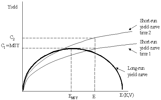
In year two, this problem is further worsened due to short run fluctuations; C₂ (assumed to be equivalent to the capacity output, given E) is not only greater than the associated long run yield for that stock, but also is greater than MSY. If an input utilization measure was calculated, however, it would likely indicate a surplus of effort and fleet size could be reduced to achieve E_MSY.

This issue underscores two points: short- and long-term capacity output and input measures should be compared to the associated relevant target; and short-term fluctuations in yield due only to short-term stock fluctuations should not drive the resulting capacity output measure. The former issue requires consideration of how a long-term capacity output measure that could relevantly be compared to long-term targets might be constructed. The latter suggests that capacity output levels should be measured over time to purge the impacts of such fluctuations.

These issues also suggest that measures of input capacity may be more reliable in measuring the extent of excess capacity than output measures. Like the issue of returns to inputs or scale, which motivated our discussion of the relationship between input- and output-oriented measures, this is at least partly driven by the point at which the measures are evaluated. Again in Figure 12, the level of combined effort (E) producing both of the estimated capacity yields (C₁ and C₂) is constant and greater than that which would be required to produce MSY (E_MSY).

Two alternatives may be developed to address the issues related to short- versus long-term measures. The short-term capacity output measures developed in the preceding sections may be compared to current target output measures, based on a path toward the long run level. Or, a longer term capacity output measure evaluated in terms of long-term stock levels may be constructed to compare to long-term target output measures. Both of these measures require imputation from the more standard measurement processes that rely on observed (short-term) data. The former requires adapting the target catch goal into a current target, but this is already the focus of most stock regeneration plans and resulting TACs. The latter requires imputing capacity output for stock levels outside the range of those observed which is somewhat more problematic, and thus less definitive, than measures based on observed relationships.

In the short term, in fisheries managed using output controls, the total allowable catch (TAC) imposed on the fishery may be assumed to represent the target output level most consistent with the current stock size and objectives of management. As a result, this is an appropriate short-term target output measure for the assessment of excess capacity and thus to be used instead of observed levels (if they differ) to construct capacity utilization measures. For fisheries managed using input controls, an estimate of the appropriate target output level will need to be undertaken using either expert opinion, or biological, bio-economic or multi-objective models of the fishery (see Section 5.4) to use as a comparison point for short-term, input-oriented capacity measures.

For imputation of long-term measures, both the numerator and denominator of the capacity utilization ratios developed in Section 3 need to be adapted. In particular, for the CU measure defined as Current Catch/Potential Catch, the numerator should instead reflect a target catch level and the denominator should be evaluated at target stock levels corresponding to this catch level. This may be accomplished for either the DEA or SPF measures discussed in Section 4, as overviewed by Kirkley, Morrison and Squires (2001).

In practice, this is not as significant an issue for input-oriented measures, since such measures are defined according to existing catch and stock levels, and thus do not impute beyond the observed data. It is still the case, however, that if long-term output and stock levels are the focal points, the long-term level of capacity consistent with the target output and stock level should be imputed for comparison purposes. If the stock is currently overfished, this may imply a higher capacity base than that associated with the given levels of catch and stock, since C_msy will exceed the current output level (or TAC). But this is likely to be more than counteracted by the greater catch per unit of K possible at higher stock levels.

5.2 Excess capacity, overcapacity and absolute capacity

The difference between excess capacity and overcapacity is not well specified in the fisheries capacity and capacity utilization literature. A useful distinction, however, is that employed by the National Marine Fisheries Service (2001). Overcapacity occurs when the potential output that could be produced, conditional on desired resource levels and full utilization of variable inputs, exceeds the level desired by management (i.e. a target level). Return to Figure 11 and assume that the desired resource condition corresponds to the resource condition producing the short-run yield curve in time two. This stock level is higher than the stock level supporting MSY. In this case, we would have overcapacity because our potential output is higher than the level needed to support our target stock level. If we further applied our weak concept of capacity output, catch or output would become bounded or limited at some point of fishing effort. That point would coincide with our potential capacity output, and the difference between output levels corresponding to that point and the point corresponding to the intersection of the short- and long-run yield curves would represent overcapacity. In contrast, excess capacity implies that, likely due to regulatory constraints, existing catch levels could potentially be taken more efficiently at existing biomass stock levels.

Since management is typically concerned about the capacity of a fishing fleet, it is important to make the distinction between excess and overcapacity. Excess capacity is essentially a short-run concept; in fact, the concept of capacity is a short-run concept. Excess capacity equals the difference between the potential output that could be produced given existing technology, resource conditions, and full variable input utilization and either the observed output or technically efficient output level (Färe, Grosskopf and Kokkelenberg, 1989).

In contrast, overcapacity has been characterized relative to desired resource conditions. As such, it is an intermediate to long-run notion, although this is somewhat inconsistent with the concept of capacity output. Overcapacity is the difference between the potential output that could be produced given existing technology, desired resource conditions (i.e. target level), and full variable input utilization, and the output level desired to support target resource conditions. Whether or not overcapacity is always a problem depends, in part, on the flexibility of the fleet to change to other fisheries. If an existing fleet of vessels operating in a particular fishery poses serious overcapacity concerns and the vessel operators have no flexibility to change to other fisheries, overcapacity will continue to pose a long-term problem. Excess capacity poses problems if it is chronic, and again, vessel operators have no flexibility to change to other fisheries. It is often the case that existing vessels cannot easily change to other fisheries, because of management and regulatory strategies.

Overcapacity also has been identified as the difference between current capacity and target capacity. That is, overcapacity (OC) might be expressed as the ratio:

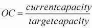
So if the target output in a fishery was 125 tonnes (based on biological and/or economic objectives), while the current capacity output was 200 tonnes, the fishery has the potential to harvest 60 percent more than the target capacity. Alternatively, such a ratio could be expressed directly in terms of capacity input levels.

This defines OC essentially as an inverse capacity utilization measure, where current capacity is expressed in terms of potential output given the current capacity base, and the comparison or reference point is target output (or, analogously, for an input measure). However, as noted prior, this comparison may be somewhat misleading since it may contain both short and long run measures, which are not necessarily comparable, and it finesses the issue of current stock dependence (i.e. comparisons of current capacity should be made in terms of current targets rather than long-run target levels). Alternatively, “current capacity” should be evaluated at long run stock levels to generate a more appropriate long-term measure of capacity (i.e. current capacity should be estimated conditional upon resource conditions necessary to support the target capacity level; for example, the population needed to yield MSY or some other objective).

The relative capacity measure specified above (OC), and implicitly (in inverse form) in the earlier discussion of CU, is also sometimes expressed in absolute terms, or levels, as:

Overcapacity = Current Capacity - Target Capacity

Overcapacity of 75 tonnes is implied for the above example.

Relative measures are usually more desirable for measuring overcapacity or excess capacity, since they are in proportional terms and measurement units are not an issue. Thus, they better facilitate identifying which fisheries (or species) are in most need of capacity management intervention. A large fishery may have a large, absolute overcapacity measure, while a small fishery may have a substantially smaller absolute overcapacity measure. However, in relative terms, the smaller fishery may have a greater overcapacity “problem” than the larger fishery. Similarly, a species with a relatively small catch in a multispecies fishery may have a small, absolute overcapacity problem but a large, relative overcapacity problem.

Finally, note that the term “overcapitalization” is often used interchangeably with overcapacity. The concept of overcapitalization directly refers to input capacity and to the level of capital stock in particular. A fishery is considered to be overcapitalized if the capital stock is greater than that required to efficiently achieve the target level of output. The existence of excess capacity generally implies overcapitalization, but it is possible to have excess capacity without having overcapitalization (e.g. too many variable inputs applied to the capital stock). In addition, a fishery can be overcapitalized even if excess capacity is not apparent, if reallocation or a different fleet configuration could take the same catch at lower cost. This is partly an issue of boat level as compared to aggregate measures of capacity and capacity utilization. Indicators of overcapitalization also often implicitly involve a cost component, which has not been factored into our technical or physical definitions of capacity and CU. These issues are elaborated further here.

5.3 Estimation of target capacity

The concepts of target output capacity and target input capacity are inextricably linked. With the exception of the long-term average yield, which can be observed directly from catch data, all other output targets require some model (explicit or implicit) of stock dynamics that make assumptions about the level and/or form (i.e. mesh size) of effort applied to the fishery. Hence, for every target output is associated a potential equivalent target input. Similarly, where fisheries are managed by controls on inputs, input targets are set on the basis of the expected output that those inputs will produce.

As just noted, the models used to determine target capacity may be either explicit or implicit. Explicit models may be either biological (e.g. MSY is the preferred target), bio-economic (e.g. MEY is the preferred target), or multi-objective (if some alternative output level is the preferred target). These models have a formal mathematical structure and are generally estimated from data. An advantage of such models is that their robustness can be tested by comparing the estimates with known events, and the structure and underlying assumptions are readily apparent and hence can be debated, agreed or disagreed. In some nations, explicit biological, bio-economic and multi-objective models have been developed that can be used for estimation of long term target output and input levels for many fisheries. On a global scale, however, neither bio-economic models nor multi-objective models have been widely used to estimate the long-term output or input levels of fisheries. Where such models do not exist, expert opinion may be sought to provide estimates of target capacity.

Implicit models are informal models that may have no foundation in existing data (possibly because such data do not exist) but may be based on observation and experience. These models have no explicit structure that can be debated and agreed upon. Such models often exist in the minds of experts, who may form opinions about how the fisheries may respond to certain changes based on their own experiences. Midway between these models are theoretical models that are based on established theory and opinion. Such models may have a formal mathematical structure but may not have sufficient data to derive the appropriate modelling parameters and conduct tests on their robustness.

5.3.1 Expert knowledge

A panel of experts may provide “educated guesses” about the level of capacity utilization and the potential harvesting ability of particular fleets, as well as estimates of target capacity (defined by the objectives of the fisheries policy or management plan) and, consequently, relative capacity. A formal technique (the Delphi Technique) has been developed that facilitates consensus between a group of individuals with expert knowledge on the issues to be examined. Tone (1999), however, offers an alternative to the traditional Delphi Technique to obtain both consensus and empirical estimates of economic parameters.

The Delphi Technique was pioneered by the RAND Corporation to gather opinions from a group of experts (Patton, 1986). A key feature of the technique is the anonymity of the participants. The experts neither meet nor know each other's identity.

The first step of the technique is to form a panel of experts and involved parties in the area of research. For the purposes of capacity estimation, this might include industry representatives as well as scientists. Information about who is on the team is not disclosed to others in the team. The basis of the anonymity requirement is that in any group of experts, it is likely that some individuals will be perceived to have had more experience than others. As a result, the opinions of these individuals may be perceived to have greater credibility than those of the others in the group. Consequently, less experienced team members might be reluctant to challenge the opinions of better known experts. Therefore, the opinion of the team would often reflect the opinion of the dominant team member and would not constitute a true, unbiased consensus. To overcome this problem, the Delphi Technique involves using a team of experts who do not know who the other team members are.

The second step is to have individuals within the team provide initial estimates (in this case, capacity, capacity utilization and target capacity) and the reasoning behind their estimates. Ideally, the participants will have some information available on current catch and activity levels, such as might be collected in a Rapid Appraisal (RA) or survey of the fishery. Participants document their opinions and supporting reasons, and return these to the group moderator. The moderator is independent of the team, and does not participate directly in the estimation of capacity (i.e. does not provide an opinion).

The moderator synthesizes the information provided by each expert into a single document outlining the estimates and reasoning of each expert. Care is taken that no comment or opinion is traceable to its originator.

The fourth step is to send a summary document to all experts for their responses. At this stage, the experts are asked to re-evaluate their estimates on the basis of the arguments proposed by other experts. The experts also are requested to propose reasons why they do not support other estimates. These responses are then sent to the moderator, who again compiles all responses into an updated summary document.

The process continues until either the experts' opinions converge or the moderator concludes that the comments have ceased to change substantively during successive rounds. In the latter case, if consensus is not achieved, the moderator must make a subjective assessment about which values to accept. At this point, greater weight may be given to the estimates of more experienced panel members, or the members who present the more convincing arguments for their estimates.

An advantage of the Delphi technique is that it works as an informal, subjective model when decisions are based on opinion, and can be directly converted to a formal model when the data are more knowledge based (e.g. based on information on catch and effort levels). However, the technique has a number of problems that need to be considered. Employing a team of experts may be expensive, and the iterative process may be time consuming. There also exists the potential for bias to be introduced (intentionally or unintentionally) by the person administering the technique (the moderator) through the summary reports presented to the group. While the group of experts does not know the members of the group, the moderator would be aware of the members and may inadvertently bias the summary towards the opinions of individuals who are perceived to be more authoritative.

An alternative process involves the use of face-to-face meetings, in which the moderator compiles the answers and presents them immediately while ensuring confidentiality. There are several computer programmes designed to assist in this process. While some anonymity and time for reflection are lost, a face-to-face meeting can provide quicker results.

Expert knowledge also can be obtained through surveys or RA. This might be useful for producing initial estimates of potential output and target capacities. However, without the potential for feedback and revision, the resulting survey-based estimates may be less reliable than those achieved through the more formal Delphi approach.

5.3.2 Biological, bio-economic and multi-objective modelling

Biological models have been developed for many fisheries around the world and underpin many fisheries management decisions. In most cases, the models are developed from commercial catch and effort data and, in some cases, supplemented with fishery independent data. The use of commercial catch and effort data requires an assumption about the relationship between catch and effort. Furthermore, such models often are used to assess the effects of different levels of fishing effort on fish stocks as an aid to fisheries management decision-making. As a result, most biological models can be used to assess both target output levels and input levels.

Bio-economic models are less common than biological models and have to date played a lesser role in fisheries management decision-making. Nevertheless, a substantial number of bio-economic models have been developed for a wide range of species in many countries, and such models provide the type of information discussed in Chapter 2. Bio-economic models provide a means to combine what is known about the biology and the fleet into a single framework for policy analysis. Generally, a bio-economic model will have a biological component that is used to estimate how the stocks may change under different levels of exploitation and an economic component that estimates how fishers may react to changing stock, price and cost conditions. The combination of these activities upon the underlying stock structure can provide an estimate of the expected level of catch and profits within the fishery. Management regulations can be inserted into the model to estimate their effects on the level of output, stock and profitability. An example of the use of a bio-economic model for the estimation of target capacity is presented in Appendix E).

Bio-economic models may have a number of applications in assessing target output and input levels. Where MSY is considered the most appropriate target output level, a bio-economic model can be used to estimate the fleet composition and size that produces the greatest economic benefits. Conversely, a bio-economic model can be used to estimate the fleet size and structure that maximizes economic benefits for the fishery as a whole, and the associated target level of output. This is particularly useful in multispecies fisheries where harvesting the MSY of individual species may lead to incompatible targets, because one “optimally” managed fishery may result in some other species being harvested above and others, below MSY.

One form of model that is particularly relevant for estimating target capacity is a bio-economic, multiobjective optimization model. Such a model is generally developed as an extension to standard bio-economic models, and includes a range of other factors associated with the fishery and fishing activity (e.g. employment level, pollution levels). Such optimization models can be used to estimate the level of output and fleet configuration that best achieves the objectives of fisheries management. This, then, can provide managers with an indication of both output-based and input-based target levels of capacity either in the long run or short run (or both in some cases). Further, optimization models also can be used to estimate the most economically efficient fleet structure to achieve the target output. Hence, they also provide information on the level of overcapitalization in the fishery. Multiple objectives of management can thus be combined into a single optimization framework to provide estimates of optimal sustainable yield that are consistent with the range of objectives usually inherent in fisheries management plans. Multiple-objective models have not been widely used to determine management and regulatory strategies for fisheries. They are often quite complex to solve, and their results are often quite difficult to apply. They do offer, nevertheless, a comprehensive framework for determining capacity output in fisheries. A recent review of the use of multiobjective programming in fisheries is given by Mardle and Pascoe (1999). A simple example of this work is presented in Appendix F.

Development of bio-economic multiobjective optimization models is a multidisciplinary task involving input from biologists, economists, fishery managers and commercial operators. Further, development of such models requires detailed biological and economic data, and constructing and validating the model can take a considerable amount of time. As a result, it is unreasonable to expect that models be developed solely for the purposes of estimating target capacity. However, because bio-economic models can be useful tools for the management of fisheries in general, States are encouraged to develop bio-economic and multiobjective models to do so. Once developed, the models also can be used to provide estimates of target capacity.