2.8 Estimation of variability factor for the use for calculation of short term intake

At its 37^th Session the CCPR decided to postpone discussion¹ on the variability factor awaiting the discussion by the 2005 JMPR.

The variability factor, as used in short-term intake assessments when estimating residues in crop units, was defined by an FAO/WHO consultation² and refined by an international conference³ as the ratio of the 97.5^th percentile of the residue population in a lot divided by the average residue of that lot. The methods of calculation were further refined by the JMPR⁴, which proposed variability factors for different types of commodities. At that time the highest residue in a crop unit, from a sample consisting of a number of crop units at or above 90, was considered to represent the 97.5^th percentile of the population in the sampled lot. This method over-estimated the variability in more than 90% of the cases, because the highest residue can be much higher than the 97.5^th percentile (P_0.975).

As part of its previous discussion, the JMPR considered the work of the International Union of Pure and Applied Chemistry (IUPAC)⁵, which also attempted to make best use of the available data, and noted that for the purposes of data analysis the IUPAC project selected only those cases where 95% or higher of the individual units had detectable residues. The initial concern was that the calculated variability would be frustrated if more than a very few of the units were non-detects. It is likely that this selection criterion ruled out most of the "mixed lot" data sets. (Attachment II - Example 2). The probability of contribution, of individual residue values, to the 97.5^th percentile was taken into account in the calculation of the best estimate for the variability factor, which led to a generic value of 3. The 2003 JMPR⁶ adopted the refined variability factor of 3 based on the scientific evaluation of all available relevant data.

The methodology referred to above^4,7,9 was developed to assess the toxicological acceptability of theoretical short-term intake of residues. The intake estimates were derived using maximum residues levels resulting from GAP reported in supervised trials.

The JMPR fully supports the conclusion of the European Food Safety Authority (EFSA) Scientific Panel regarding the unsuitability of monitoring data, based on sample size specified in the Codex sampling procedure and the EU homogeneity studies for estimating variability factor.

The JMPR IESTI procedure should only be used for estimation of short-term intake from residues found in crop units taken from a single lot as defined in the Codex sampling procedure.

It is not applicable for residue data obtained from market samples, where the commodities offered for sale are of mixed lots, which may result in a variability factor three to four times higher than the one in the treated lot (Attachment II, Example 1). Consequently, it is not appropriate to attempt to derive a variability factor using residue data of uncertain origin or those clearly indicating that the sampled commodity originated from a mixed lot, i.e., a high CV value, in the estimation of short-term intake based on data from supervised trials.

The JMPR considered the results of the new studies coordinated by the Joint Division of FAO and the International Atomic Energy Agency (IAEA) ⁷ (summarized in Attachment I) and the data base which was used for preparing the opinion of the EFSA Scientific Panel⁸.

The FAO/IAEA project resulted in 11 112 valid residue data in crop units from 13 countries of 3 continents representing 3 small fruits, 5 large crops, 2 medium/large crops and 3 leafy vegetables, and included 25 pesticide active ingredients. Evaluation of these new residue data and the relevant supervised trials (3 new and 8 evaluated previously) carried out by the pesticide manufacturers resulted in an overall average variability factor of 2.8 (IUPAC procedure) and 2.7 obtained with the Harrell-Davis method used by the EFSA Scientific Panel. The values correspond with the average factor (2.8) obtained by EFSA for medium size crops based on supervised trials. Due to the inevitable random nature of the variability factor derived from the combined uncertainty associated with sampling and analysis (Attachment II. Example 3), the best estimate of the variability factor can be gained be meaning the variability factors derived from samples of various crops⁹. This approach was also followed by IUPAC⁸.

In order to ascertain the suitability of the variability factor of 3 as currently applied by the JMPR, all data used by the EFSA Scientific Panel, and the new data provided by FAO/IAEA and derived from recent supervised trials, were evaluated. A simple procedure was used and did not apply any prior assumptions. The residues (R_i) measured within an individual data set were divided by the average residues, R_ave, of that particular data set. The instances where the ratio was found to be higher than 3 was then recorded. The results are shown below:

(a) These data do not include the EPCA grape and lettuce trials with tank mix of pesticides because they were taken into account in the evaluation of the data obtained from the FAO/IAEA Project.

(b) 4 grape and 4 lettuce data sets from the ECPA trials from France and Germany are included in this summary. In the latter case, trials giving the highest variability factors from the tank mix pesticides were selected.

The number of cases where the ratio was higher than 3 provides a measure for the suitability of the current default variability factor of 3 used by the JMPR.

The analysis of all supervised trials and market surveys data available (191 data sets, and 22,665 residue data from crop units) indicated that the R_i/R_ave ratio exceeded 3 for only 2.45% of the residue data. The very large amount of actual residue data does not support the conclusion of the EFSA Scientific Panel stating that: variability factors for supervised trials and market surveys will exceed the proposed default value of 3 in 34% and 65% of cases, respectively. In fact, 7002 market samples indicated that only 4.2% of crop units contained residues for which the ratio (R_i/R_ave) exceeds 3, and the field and supervised trials (15,663 residue data) gave R_i/R_ave ratio > 3 in less than 1.7% of cases.

Taking into account the new residue data and the existing data, suitable for estimating the variability factor as well as the applicability of the IESTI calculation, the Meeting concluded:

• Since theoretically 2.5% of the R_i/R_ave values could be above 3 and actually 2.45% of all measured residues exceeded the value of three times the average residue, the current JMPR default value of 3 is a good estimate for the variability factor. That it effectively covers the practical variability of residues likely to be found in a wide range of medium and large sized commodities (fruits and vegetables), and can be used to provide the best estimate currently possible for the short-term intake at the international level.

• The best estimate of the variability factor can be gained from the average of the variability factors calculated for individual crop samples. As the variability factor is estimated at 95% confidence level, it is not appropriate to apply an additional confidence or credibility limit over it.

The JMPR agreed to continue using the default variability factor of 3 for calculation of IESTI, which will be expressed with one significant figure corresponding to its uncertainty.

It is emphasized that the deterministic IESTI calculation used by JMPR should only be applied to residue data derived from supervised trials and single lots. It is not applicable for mixed lots.

ATTACHMENT I

Summary of studies carried out for determining pesticide residues in crop units

When estimating the short-term intake of pesticide residues the variability of the residues in crop units is taken into account. As the vast majority of residue data available was on medium sized crop commodities, the Joint Division of the FAO and the International Atomic Energy Agency (IAEA) initiated a coordinated research programme³ to undertake field studies to investigate residues in individual items of leafy vegetables as well as small and large crops. The aim being to provide residue data to enable the refinement of the estimates of the variability factor and the uncertainty of associated with sampling.

The results of the project and the relevant data from supervised field trials carried out by the European Crop Protection Association¹⁰, (ECPA), and the company BASF¹¹ are summarized below.

Within the FAO/IAEA Project field trials were carried out in 13 countries on 13 commodities including 3 small fruits, 5 large crop commodities, 2 medium/large crop commodities and 3 leafy vegetables. The 25 pesticide active ingredients applied represented the dicarboximide (3), organophosphorus (8), synthetic pyrethroids (5), phthalimides (2), organochlorine (1) and other types of pesticides (6). The crop pesticide combinations amounted to 91 combinations, from which 6,116 samples were analysed resulting in 11 112 valid residue data.

In addition, supervised trial data provided by BASF on grapes in Germany and Spain, and 4 grape and 4 lettuce data sets from the ECPA trials from France and Germany are included in this summary. In the latter case, trials giving the highest variability factors from the tank mix pesticides were selected taking into account the conclusion, reached by the EFSA Scientific Panel¹, that the variability factors obtained from a set of pesticides applied in a tank mix may not be independent. These supervised trials included 7 different pesticides analysed in 1320 samples.

The FAO/IAEA field trials represented regular agricultural practice prevailing in different parts of the world, e.g., Europe, Latin and Central America and South-East Asia. They were performed on commercial fields cultivated and treated with pesticides by local farmers as per normal practice. The samples were collected by trained personnel who followed detailed sampling plans. The samples were then analysed using validated methods of known and acceptable performance parameters.

The recoveries obtained during method validation generally ranged between 75 and 110%. In a few cases lower (minimum 63%) and in one case higher (121%) average recoveries were reported. The laboratory reproducibility values, including the error of sample processing CV_L values, were within the acceptable range according to the CCPR GLs¹². The internal quality control measures confirmed that the analyses of the samples were carried out properly and produced reliable and accurate results.

As the field trials represented normal agricultural practice, based on the performance of the methods it can be concluded that the results reflect the variability of residues to be expected in commodities available in single lots in the market. The results provide a good and reliable basis for estimation of the variability of residues in crop units treated in field trials.

Data sets usually contained detectable residues. In a few cases, where residues < LOQ values were present (< 10%), they were substituted with the half of the lowest reported value only if the replacement did not result in more than 10% difference in the mean residues or the coefficient of variation of the residues, CV_R. The replacement should not significantly affect the estimated CV_R and the variability factor.

Due to the inevitable random nature of the variability factor deriving from the combined uncertainty of sampling and analysis, the best estimate of the variability factor can be gained from the average of the variability factors calculated from samples of various crops¹⁰. This approach was also followed by Hamilton et al. 2004⁸.

The results are summarized in Table 5. Details of the experimental data will be published elsewhere¹³.

Table 5. Summary of variability factors for various commodities

^1. Variability factor calculated from the 97.5^th percentile/average residue obtained with Excel programme.

^2. Variability factor calculated according to Hamilton et al. 2004.

^3. Variability factor calculated with the Harrell-Davis method applied by the EFSA Scientific Panel.

^4. Fruits (average single increment mass 40-225g) were collected from close vicinity to represent approximately the large portion size used in short-term exposure assessment.

ATTACHMENT II: EXAMPLES.

1. Variability of residues in mixed lots/

Experimental data sets were used to illustrate the effect of mixing lots.

Let's assume that the two kale lots treated with indoxacarb (lot 22 and 49) and two grape lots (20 and 17) treated with chlorpyrifos would be mixed with each other, and the grape lot 17 containing 2.37 mg/kg residue would be mixed with untreated fruits in 1:1, 1:2 and 1;3 ratios. The effect of mixing is illustrated in Table 6.

Mixing commodities treated with the same pesticide results in a variability between the two lots, while mixing a treated commodity with untreated one will increase the apparent "variability factor". The larger the residue concentration in the treated lot and lower the LOQ, the larger will be the new variability factor. Similarly the rate of dilution with untreated commodity will approximately proportionally increase the "variability factor".

Table 6. Effect of mixing commodities on the variability factor

^#Grape 2 lot was mixed with other grape lots that did not contain any residue

2. The effect of non-detects on variability of residues

The criterion chosen to minimize the effect of non-detects on the calculations was to make the calculations twice, once with the non-detects = 0 and once with non-detects = LOQ (limit of quantification). If the difference in the calculated variability factor was less than 10%, the data set was accepted (cf. page 18 of EFSA report). This criterion would accept mixed lots, e.g. it would accept a mixture of 90% untreated commodity (LOQ = 0.01 mg/kg) with 10% of treated commodity (residue level = 1 mg/kg).

The summarized data from the 69 relevant data sets in Appendix II of the EFSA paper were examined for the relationship between estimated variability factor and percentage non-detects (Table 7). The estimated values for variability factors appear to be influenced by the percentage of non-detects (when more than about 10%), which suggests either a problem with the calculation method or that these data sets are really mixed lots and the estimated variability factors are not relevant for true lots.

Table 7. The effect of non-detects, and possibly mixed lots, on the estimated variability factor.

3. Illustration of uncertainty resulted from sampling

To illustrate the variability of the estimated parameters, large test populations (T1-T7) were created from the available residue data.

The parameters of the test populations are given in Table 8. The test populations have variability factors ranging from 2 to 4.6, which cover the range that is likely to occur in practice.

Table 8. Characteristic parameters of the test populations

¹ Rescaled populations from measured residues.

² The data points are the back-transformed values from a log-normal population derived from original experimental data.

³ Combined residues from data sets of the same commodity

⁴ Calculated with Excel

⁵ Calculated with Harrell Davis method

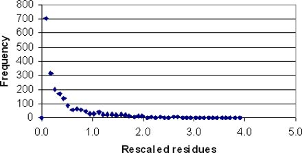
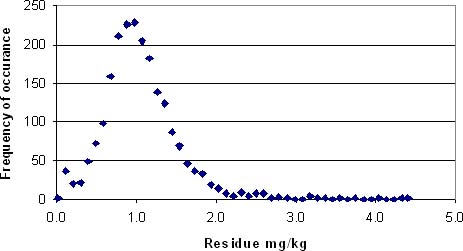
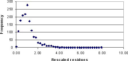
The distribution of residues in the test populations are illustrated in Figures 4 to 6, and show that they are quite different in shape, thus accurately represent the situations that may occur in practice.

Random samples of size 100-120 and 200 were drawn (1000 from each population) from the test populations with replacement. The results indicating the range of estimated variability factors due to the sampling uncertainty are shown in Table 9.

Figure 4. The distribution of residues in the T-2 test population.

Figure 5. The distribution of residues in the T-3 test population.

Figure 6. The distribution of residues in the T-4 test population.

Table 9. The relative 95% confidence limits for P0.975/Rave

LCL_0.025 lower confidence limit, UCL_0.975 upper confidence limit

The percentage deviation of the minimum and maximum variability factors from the mean observed based on 1000 replicate samples in the test populations, is in the similar range and reflects the random variation derived from sampling uncertainty.

The 95% relative confidence intervals of the variability factors estimated from samples of size 100 are practically independent from the variability factors of the parent populations and they are on average in the range of 9% to 40%. This means that an observed range of 2.7-4.2 for a variability factor of 3 can be attributed to the sampling uncertainty at 95% probability level.

References:

1. Codex Secretariat, Report of the 37^th Session of the Codex Committee on Pesticide Residues, Alinorm 05/28/24

2. WHO, 1997. Food consumption and exposure assessment of chemicals, Report of a FAO/WHO Consultation, Geneva, Switzerland, 10-14 Feb, 1997, Document WHO/FSF/FOS/97.5 (1997).

3. PSD, 1998. Report of the International Conference on Pesticide Residues Variability and Acute Dietary Risk Assessment. The Pesticides Safety Directorate, York, UK, 1-3 Dec 1998.

4. FAO. Pesticide residues in food. Report of the Joint Meeting of the FAO Panel of Experts on Pesticide Residues in Food and the Environment and the WHO Expert Group on Pesticide Residues. Chapter 3. FAO Plant Production and Protection Paper 167, Food and Agriculture Organization. Rome, (2001).

5. Hamilton D.J., Ambrus A., Dieterle R.M., Felsot A., Harris C., Petersen B., Racke K., Wong S-S., Gonzalez R. and Tanaka K. Pesticide residues in food - Acute dietary Intake, Pest. Manag. Sci. 60, 311-339. (2004).

6. FAO. Pesticide residues in food. Report of the Joint Meeting of the FAO Panel of Experts on Pesticide Residues in Food and the Environment and the WHO Expert Group on Pesticide Residues. FAO Plant Production and Protection Paper Food and Agriculture Organization. Chapter 3. Rome. 2004.

7. Development of Sampling Guidelines for Pesticide Residues and Strengthening Capacity to Introduce Certification Systems, PFL/INT/856/PFL - 111740

8. EFSA, Opinion of the Scientific Panel on Plant health, Plant protection products and their Residues on a request from the Commission related to the appropriate variability factor(s) to be used for acute dietary exposure assessment of pesticide residues in fruit and vegetables, EFSA Journal 177, 1-61, 2005.

9. Ambrus Á. Within and between field variability of residue data and sampling implications. Food Additives and Contaminants 17(7): 519-537. (2000).

10. FAO, Pesticide residues in food. Report of the Joint Meeting of the FAO Panel of Experts on Pesticide Residues in Food and the Environment and the WHO Expert Group on Pesticide Residues. Annex 7, FAO Plant Production and Protection Paper 172, Food and Agriculture Organization. Rome, (2002).

11. Regenstein H, Personal communication, 2005.

12. Codex Secretariat, Revised Guidelines on Good Laboratory Practice in Residue Analysis ftp://ftp.fao.org/codex/alinorm03/al03_41e, 2003.

13. Ambrus Á. Variability of pesticide residues in crop units (Submitted for publication in Pest. Manag. Sci.)

2.9 Estimation of Processing factors

Processing studies are among the critical supporting studies required for the evaluation of new and periodic review compound.

The FAO Manual (2^nd edition p. 44) specifies the procedure which has been followed by the FAO Panel. It provides the following options:

a. If more than one processing study has been conducted for a particular pesticide in the same raw agricultural commodity (RAC), the average processing factor for each type of process should be used for each processed commodity.

b. If the processing factors from two trials are irreconcilable, e.g. 10-fold different, the mean is inappropriate because it would not represent either process, then the highest processing factor should be chosen as the default (conservative) value if there is no other reason to choose one or the other.

c. If residues in the processed commodity are undetectable or < LOQ in several studies it may mean that residues in the processed commodity are very low or essentially 0, and the calculated processing factor is merely the reflection of the starting residue level in RAC In this case the best estimate of the processing factor is the lowest "less than" value rather than the mean of the "less than" values.

There are certain cases which are not covered in the above examples

1. Processing studies may result in processing factors including both "less than" and real values, or some high values without any identifiable reasons. In such cases the median value should be taken as the best estimate as the calculation of the mean provides a biased value.

2. Processing factors are determined from the RAC at various days after the last application. In this case the results from the shortest PHI onward should be taken into account. An example is the processing of grape treated with fenhexamid to wine.

As the processing factors are not different all data can be considered and the mean or median values could be used as best estimate for the processing factor.

3. However, in cases where the difference between the median and the mean is larger than 20%, the distribution is not close to normal so the median of the valid values would provide the best estimate.

Consequently the median would generally provide the best estimate for the processing factor, and the Meeting decided to use it instead of the average value in the evaluations of the processing studies.

2.10 Definition of fat-soluble pesticides in meat and fat

Revisited: Fat-soluble pesticides in meat and fat

As part of the JMPR guidance regarding fat-solubility, physical chemical properties and definition of the residue,^[2] one of the factors that should be considered when proposing a residue definition is the fat solubility of the compound and relevant transformation products. Due to a number of fat-soluble compounds being reviewed at this meeting, and in addition to the guidance from the 2004 Meeting regarding MRLs for fat-soluble pesticides in milk and milk products, it was considered timely to revisit the criteria that are important when designating a residue as 'fat-soluble'. A 'residue' is defined as the combination of the pesticide and its metabolites, derivatives and related compounds to which the MRL or STMR apply^[3].

The designation of a residue as either 'fat-soluble' or non-fat soluble is important for trading purposes and compliance with relevant standards. In trade situations where meat products are sampled at export destinations, the residues of a fat-soluble pesticide measured in meat may be inconsistent due to muscle samples containing different levels of interstitial fat either within a single animal, i.e. a single carcass, or in different animals. From a compliance perspective, it is better to regulate on the residue in the trimmable fat component of the meat, as the residue will be more consistent in fat, when compared to muscle. The 'fat-soluble' status determines the nature of a sample that should be taken for enforcement analysis.

The expression of MRLs for fat-soluble pesticides in meat and animal fat was considered by the Meeting in 1991 and published in a general considerations item^[4]. The JMPR chose the octanol-water partition coefficient as the physical property that could indicate solubility of a compound in fat and the Meeting examined a number of compounds with MRLs in animal commodities and their respective P_ow values where they were available. The recommendations of the 1991 Meeting were:

The octanol-water partition coefficient (log P_ow) should be the prime indicator of fat-solubility, supplemented by inferences that may be drawn from the distribution of residues between muscle and fat tissues, when the residue consists of a single compound.

In cases where the residue is defined as a mixture of the parent compound and metabolites, information on the log P_ow of the individual compounds should be considered if available.

In general, when log P_ow exceeds 4, the compound would be designated fat-soluble and when log P_ow is less than 3 it would not be so designated.

The partitioning of residues between fat and muscle as a function of P_ow can be predicted. A plot of log P_ow versus predicted partitioning in meat between fat and muscle reveals that partitioning is essentially independent of log P_ow for compounds with values greater than 3. The Meeting decided to revise the empirical limits recommended by the 1991 JMPR when considering log P_ow so that when no evidence is available to the contrary and log P_ow exceeds 3, the compound would be designated fat-soluble and when log P_ow is less than 3 it would not be so designated.

The partition constant k for fat and muscle (see Figure 7) can be calculated assuming P_ow (octanol:water) has the same value as P_lw, the partition constant for lipid and water. Further, if it is assumed that muscle contains 5% lipid with the remainder water and that fat is 100% lipid then: P_lw = [lipid]/[water] » P_ow; k = [fat]/[muscle]; k = [lipid]/(0.05*[lipid] + 0.95*[water]); k = (1-x)/{0.05*(1-x) + 0.95*x)} where x = 1/(1+P_ow).

Figure 7. Plot of predicted variation in partitioning in meat based on log P_ow and fat content.
In general, when log P_ow exceeds 4 the compound would be designated fat-soluble and when log P_ow is less than 3 it would not be
It is stated in the FAO Manual (2002):

Fat solubility is a property of the residue and is primarily assessed from the octanol-water partition coefficient and the partition of the residue between muscle and fat observed in metabolism and farm animal feeding studies. ... Sampling protocols for animal commodities depend on whether a residue is fat-soluble or not [p52].

so designated. Pesticides with intermediate log P_ow would be considered on a case-by-case basis using the evidence of residue distribution between muscle and fat tissues [p40].

Some worked examples are provided for recently reviewed compounds with log P_ow >3 to illustrate different situations and the determinants that may be used to define a residue as being fat-soluble or not fat-soluble for the purposes of JMPR and the estimation of maximum residue levels for meat. Only goats and cattle are considered here, however the same principles apply to hen studies and poultry.

Residue concentrations for the residue definition in both muscle and fat may be compared in the goat metabolism study, where the data allow. These values are compared to the residue concentrations found in the muscle and fat in the corresponding cattle feeding study, and the ratio between muscle and fat may be compared. Data for milk and milk fat may also be considered as an additional factor regarding the fat solubility of a pesticide, although in some instances the residue may be designated fat soluble in meat but not in milk due to differences in partitioning of the individual components included in the residue definition. Examples are discussed below.

Cyprodinil has a log P_ow = 4, the residue is defined as parent compound. The residue in goat fat is 75 × higher than the residue in muscle in the metabolism study, indicating greater solubility of the residue in fat versus muscle (2003 JMPR). On the basis of the data from the metabolism study, the residue is designated as being fat-soluble.

Flutolanil has a log P_ow = 3.17 and the residue is defined as the sum of flutolanil and trifluoromethyl benzoic acid for animal commodities. The cattle feeding study indicates that the residues in muscle and fat are comparable (2002 JMPR). On the basis of the data provided, the residue as defined for flutolanil is designated as not being fat-soluble.

Haloxyfop-R-methyl ester (active form) has log P_ow = 4; haloxyfop methyl (racemate) log P_ow = 3.52; haloxyfop acid log P_ow = 1.32; the residue of haloxyfop is defined as haloxyfop esters, haloxyfop and its conjugates expressed as haloxyfop. Results from two cattle feeding studies have been reported by the JMPR (1996, 2001); the first by the 1996 JMPR showed residues in fat are higher than in muscle while the second reported by the 2001 JMPR showed residues in fat and muscle were comparable. The results can be explained by the analytical methods utilized in the two studies. Metabolism studies showed haloxyfop was present in fat as a non-polar conjugate that is easily hydrolysed under alkaline conditions to yield haloxyfop; in milk fat the conjugates were identified as conjugates of triacylglycerols. The cattle feeding study reported in the 1996 JMPR utilized an alkaline hydrolysis step to extract residues from all tissues while the later study utilized base extraction for muscle, kidney and liver but not fat. An alkaline extraction is an integral part of the analytical method for both plant and animal matrices and it is clear that the later study reported by the 2001 JMPR should be discounted. On the basis of the cattle feeding study where both fat and muscle samples analysed using an appropriate residue method, the residue should be designated as fat-soluble. This conclusion differs from the recommendation of the 1995 JMPR.

Fipronil has a complex residue definition and the log P_ow for fipronil is 3.5 and log P_ow for a primary metabolite (MB 46136) is 3.8. The residue concentrations (parent + MB 46136) are 20 to 30 × higher in goat fat compared to muscle in the metabolism study (2001 JMPR). In the cattle feeding study, residues (fipronil and MB 46136) were not detected in muscle (< 0.01 mg/kg) following dosing at the equivalent of 0.43 ppm. The individual components of the residue in fat were 3 to 4 × higher for fipronil and were 40 to 50 × higher for MB 46136 than those in muscle (< 0.01 mg/kg). Following combined dermal and oral administration to cattle, levels of fipronil and MB 46136 were < 0.01 mg/kg in muscle, however fipronil levels in fat were 4 to 6 × higher than the muscle LOQ and levels of MB 46136 ranged from 7 to 77 × higher than the muscle LOQ over three fat depots sampled. The data clearly show that the residue as defined (fipronil and MB 46136) is fat-soluble. As is often the case, there are significant differences in residue levels in renal fat compared to abdominal fat illustrating the need for individual fat depots to be analysed in cattle feeding studies.

The above examples demonstrate that log P_ow of an individual component of a residue is an initial indicator, however it is not the only factor used to assess fat-solubility.

The considerations applied to the designation of a residue definition as fat soluble or not for meat and fat should also be utilized in the design of any livestock feeding study. Data generated in a livestock study (radiolabelled or transfer) should adequately demonstrate that consideration of the fat-solubility of the chemical and/or metabolites has been taken into account. If the study is not adequately designed, and appropriate samples have not been taken, then it may be difficult to determine whether a residue should be designated as fat-soluble. In addition, if adequate sampling of different fat depots has not taken place, it may be difficult to determine whether MRLs have been recommended at appropriate levels. For the purposes of study design, any residue (compound and/or metabolites) with log P_ow> 3 should be considered as potentially being fat-soluble.

The Meeting recommended that in determining "fat solubility" for a residue the following factors should be considered:

• When available, it is the partitioning of the residue (as defined) in muscle versus fat in the metabolism studies and livestock feeding studies that determines the designation of a residue as being "fat soluble".

• In the absence of useful information on the distribution of residues in muscle and fat, residues with log P_ow > 3 are likely to be "fat soluble".

The Meeting noted that in the design of animal feeding studies, account should be taken of the likely fat solubility of residues with log P_ow > 3

The Meeting also recommended that the FAO Manual be amended as follows to reflect the above discussion:

Page 40 of the FAO Manual:

The solubility of the pesticide is especially of great interest, as the ability of the compound to penetrate plant and animal tissues is dependent on its solubility in water and organic materials.

The JMPR recommended that the distribution of the residue between muscle and fat obtained from livestock metabolism and feeding studies should be the prime indicator of fat-solubility. In some cases the information available on distribution of the residue (parent compound and/or metabolites) from metabolism or feeding studies does not allow an assessment of fat solubility to be made. In the absence of other useful information, the physical property chosen by the JMPR to provide an indication of solubility in fat is the octanol-water partition coefficient, usually reported as log P_ow.

It should be noted that there are errors in estimates of log P_ow, with differences of one unit for the same compound being reported. Different approaches to the development of these data often give different results. Interpretations must recognize these differences.

The variable composition of some residues, e.g. where the residue is defined as a mixture of parent and metabolites, presents a problem since the fat-solubilities of the metabolites may be different from those of the parent compound. In this case, information on the log P_OW of each individual metabolite should be considered if available. The relative concentrations within the mixture are also subject to change and, as a result, the tendency of the mixture to partition into fat will also change.

When no evidence is available to the contrary and log P_ow exceeds 3, the compound would be designated fat-soluble and when log P_ow is less than 3 it would not be so designated.

Page 52 of the FAO Manual:

Fat-solubility is a property of the residue and is primarily assessed from the octanol-water partition coefficient and the partition of the residue between muscle and fat observed in metabolism and farm animal feeding studies. The section in this chapter, "Physical and chemical properties" provides guidelines for deciding whether a pesticide is fat-soluble. Sampling protocols for animal commodities depend on whether a residue is fat-soluble or not.

The JMPR, for many years, included the qualification "fat-soluble" in the definition of the residues of fat-soluble pesticides, using the expression:

"Definition of the residue: [pesticide] (fat-soluble)"

The 1996 JMPR recommended that "fat-soluble" should no longer be included in the definition of the residue because "fat-soluble" is a qualification of sampling instructions and is not relevant to the dietary intake residue. In order to avoid confusion while conveying the information that a residue is fat-soluble, the JMPR agreed that a separate sentence should indicate that the residue is fat-soluble.

The definition of residues has not always been consistent with these principles, which were first published in the 1995 JMPR Report with a revision published in the report of the 2005 JMPR. Therefore, all residue definitions are re-examined during the periodic review of the compounds.

2.11 JMPR recommendations for animal forage

Pesticides are needed in the production of animal forage and fodder crops, so residues in the resulting forage and fodder may be expected.

The succulent or high-moisture stages of the crop are known as forage and mostly are grazed directly or are cut and fed to livestock without delay. Examples are: maize forage, alfalfa forage and pea vines.

The dry or low-moisture stages of the crop are known as hay, straw or fodder, which may be readily stored and transported as commodities of trade.

In the past, JMPR has recommended MRLs for forage crops and has used information on their residue status in estimating farm animal dietary burden.

Codex MRLs are used as standards for commodities in international trade. The Meeting was of the opinion that forage was not an item of international trade requiring Codex MRLs and decided not to recommend further forage MRLs.

Fodder MRLs would continue to be evaluated and recommended as previously.

Forage residue data would continue to be evaluated and used in the estimation of farm animal dietary burden.

2.12 Response to CCPR regarding the ARfD for carbaryl

At the 37^th Session of the CCPR in April 2005, the Australian delegation had raised concern regarding the ARfD for carbaryl established by the JMPR in 2001. The Australian delegation had disagreed with the choice of pivotal study used for setting the ARfD and requested that JMPR review the basis for the ARfD established.

The evaluation of carbaryl by the JMPR

In 2001, the Meeting established an ARfD of 0.2 mg/kg bw based on a NOAEL of 3.8 mg/kg bw per day identified on the basis of inhibition of cholinesterase activity observed at 10 mg/kg bw per day in a 5-week dietary study in dogs, and with the application of a 25-fold safety factor.

The Australian evaluation of carbaryl

The current Australian ARfD of 0.01 mg/kg bw is based on a NOEL of 1 mg/kg bw per day identified on the basis of behavioural indications of autonomic neurotoxicity, and inhibition of brain and plasma erythrocyte cholinesterase activity in a study of developmental toxicity and a 13-week study of neurotoxicity in rats, and using a 100-fold safety factor.

When setting an ARfD for carbaryl, Australia's Office of Chemical Safety (OCS) examined the evaluation made by the JMPR and did not agree with the selection of the pivotal study. The OCS noted that Hayes & Laws (1991) had reported overt acute cholinergic toxicity in a human receiving carbaryl as an oral dose at approximately 2.8 mg/kg bw, a dose that is lower than the NOAEL of 3.8 mg/kg bw per day identified on the basis of inhibition of erythrocyte and brain cholinesterase activity in dogs, which was used as the basis for the JMPR evaluation.

Comments made by the JMPR

In the case of carbaryl, the Meeting noted that the current ARfD of 0.2 mg/kg bw is appropriate and sufficiently protective because it is one-fourteenth of the effect level reported by Hayes & Laws in a study in a single human. The Meeting noted that in general a study based on only one human individual should not serve as the basis for an ARfD, although such a case study may provide supporting information.

In the JMPR toxicological evaluation, it is stated that cholinesterase activities in dogs and rats are considered to be equally sensitive to inhibition by carbaryl. Although the NOAEL of 1 mg/kg bw per day reported in the 13-week study in rats is lower than the NOAEL of 3.8 mg/kg bw per day reported in the 5-week study in dogs, an overall NOAEL was identified by selecting the highest NOAEL below the lowest LOAEL to account for differences in dose spacing in these two studies. Furthermore, inhibition of cholinesterase activity is a sensitive and quantitative biochemical end-point that is adequately protective for other end-points, including neurological symptoms and signs. Lastly, the 25-fold safety factor that was applied to the NOAEL for inhibition of cholinesterase activity in dogs includes an interspecies extrapolation factor that would allow for a fivefold greater sensitivity of humans.

2.13 Joint FAO/WHO Meeting on Pesticide Specifications

The Meeting was informed about the work and the new working procedure of the Joint FAO/WHO Meeting on Pesticide Specifications (JMPS), and briefly discussed two examples of existing FAO Specifications and Evaluations for Plant Protection Products^[5]. The Meeting recognized the importance of this activity in developing specifications for the active ingredients of pesticides.

The Meeting considered that it is important to coordinate the activities of the JMPR and the JMPS as far as possible. Therefore the Meeting reiterated the conclusions of the 1999 Meeting, that specifications for the technical material should be developed for a pesticide before it is evaluated within the periodic review programme of the CCPR and for new pesticides, but that this should not delay evaluation of pesticides by the JMPR. The Meeting recognized that there are many compounds on the JMPS agenda that will not lead to residues in food and will therefore not be evaluated by JMPR.

The Meeting noted that the FAO Specifications and Evaluations for Plant Protection Products include sections entitled "Hazard summary" and "Appraisal", which include toxicological information and an appraisal of the hazard potential of the compound. The Meeting expressed concern that the basis for this information and whether the appraisal is a peer-reviewed evaluation of the available information is not indicated in these sections. The Meeting suggested that it should be clearly indicated whether these sections are based on existing national/regional or international evaluations.

The Meeting recommended that if JMPR evaluations exist for a particular pesticide, toxicological information from the summary tables and toxicological evaluations of the JMPR report should be used as the only entry in the relevant toxicological parts of the specifications.

The 2005 JMPR agreed to refer to available JMPS specifications in the JMPR report. However, this reference is not an endorsement of the toxicological information therein (except for JMPR hazard assessments).

2.14 Project to update the Principles and Methods for the Risk Assessment of Chemicals in Food

The Meeting briefly discussed the recommendations of the recently held workshop on exposure assessment. This workshop was part of the joint FAO/WHO Project to Update the Principles and Methods for the Risk Assessment of Chemicals in Food, and considered methods for exposure assessment of food chemicals, including pesticide residues, in relation to long-term and acute exposure.

In this context, the advancement of the 13 GEMS/Food cluster diets was discussed. The final cluster diets would be presented at the next Codex Committee on Food Additives and Contaminants (CCFAC) and CCPR meetings, and could be implemented at the next JMPR. The RIVM offered assistance in updating the calculation spreadsheets that the JMPR uses in the dietary risk assessments to replace the current five GEMS/Food regional diets with the 13 cluster diets. This was welcomed by the Meeting.

The Meeting was informed of the next steps of the project, which included a workshop to review current methods for setting MRLs for pesticide residues and veterinary drug residues, and harmonizing to the extent possible. The workshop would be held in November 2005 in the Netherlands, with the support of the RIVM.

A meeting of the Steering Group would be held early next year to review progress on the project, and a final expert consultation to review the final document of the whole project was being planned, as recommended by the Joint FAO/WHO Expert Committee on Food Additives (JECFA). Funding for such a final consultation was currently being sought.

2.15 IPCS Framework for Analysing the Relevance of a Cancer Mode of Action for Humans

The Meeting briefly discussed the draft International Programme on Chemical Safety (IPCS) document IPCS Framework for Analysing the Relevance of a Cancer Mode of Action for Humans^[6]. To promote the use of mechanistic data, the Meeting noted that the approach laid out in the document should be used in JMPR evaluations. Thus the Meeting recommended that the Secretariat should advise the JMPR Temporary Advisers to use the IPCS framework as guidance in their evaluations of cancer modes of action as appropriate.

The Meeting was informed that the IPCS document would be accompanied by case studies, to illustrate the approach to be used, and that IPCS was encouraging the submission of further examples to be included.

The next planned activity within this project would be to expand the mode of action framework to encompass end-points other than cancer.

2.16 Probabilistic modelling of acute dietary exposure

The Meeting noted the conclusions of the 37^th Session of CCPR on the proper risk management concerning the safety of Codex MRLs, which was (ALINORM 05/28/24 para 76, italics added):

'The Committee concluded that food containing residues at the level of the adopted Codex MRL must be safe for the consumers and that the Committee retains the current policy i.e., when the JMPR notes an ARfD exceedance, the MRLs are not advanced to a higher Step of the Codex Procedure.'

The Meeting reflected that to assess the safety of residues at the level of the adopted Codex MRL the development of probabilistic methodology for JMPR purposes is unnecessary. The deterministic IESTI calculation currently used by JMPR is adequate to determine whether the ARfD might be exceeded. In the IESTI a fixed residue value representing the level of the Codex MRL is combined with a fixed consumption figure, representing a large portion of the commodity being assessed. The large portion is defined as the highest large portion reported from any of the Codex Member States that provided data to GEMS/Food and is represented by the 97.5^th percentile of consumption-days only.

However, the Meeting noted that the GEMS/Food consumption database for acute exposure assessments as currently used in the calculations has limited information on the 97.5^th percentiles of consumption. Only a few countries have supplied this information to GEMS/Food, and it is not known whether all of them have derived this percentile in the same way.

For example, some countries may have reported the 97.5^th percentile consumption of fresh apple only, while others may have included the consumption of apple juice and apple in other foods, e.g. apple pie. Furthermore, to be able to assess the validity of the data provided, there should also be available a list of 97.5^th percentiles of consumption figures and the number of person-days behind this percentile, together with more information on the distribution (e.g. geometric mean and geometric standard deviation, or list of percentiles, or preferably all individual data). If a national survey does not contain enough data on a particular commodity to discriminate the 97.5^th percentile of consumption, this should be noted.

The Meeting recommended that GEMS/Food and Codex Members put more effort into refinement of the short-term consumption database currently used by JMPR, since anomalies and missing data often cause problems for the IESTI calculations.

2.17 Risk analysis principles

At the request of the Joint Secretariat, the Meeting provided comments on the Proposed Draft Risk Analysis Principles applied by the Codex Committee on Pesticide Residues (ALINORM 05/28/24, Appendix XIII). The current draft was considered to be a concise and accurate description of the tasks assigned to JMPR.

The Meeting stressed that JMPR's contribution to risk analysis is based solely on science whereas the consideration of other legitimate factors relevant to the health protection of consumers and for the promotion of fair practices in food trade is the responsibility of CCPR.

The Meeting also noted that it will continue to propose MRLs for plant and animal commodities based on the available data related to registered uses that reflect national GAPs. The decision whether an adopted CXL for a commodity shall be revoked although sufficient data are available to recommend a MRL, is the responsibility of CCPR, not JMPR.
Assessment of risk from long-term dietary intake