![]()
![]()
![]()
Fish has been a major commodity in trade for more than a thousand years and seafood trade has influenced living conditions and policy decisions for just as long. An important characteristic for all food products that are traded is that they must be transportable and conservable for at least the transportation time.[3] The traditional fish trade has therefore depended on dried or dried and salted products since these were the best traditional preservation methods, and also because they reduce the weight of the fish substantially. However, even though there has been a substantial trade with fish for a long time, in most places local fishermen were the most important providers of fish particularly to the most valuable market - the local market for fresh fish. Hence, historically even for the same species, separate local and regional markets have existed, and where prices have been determined by local supply and demand. Abundance of fish and low prices in one market was not reflected in prices on other markets. This has made the seafood market highly segmented, so that it is more relevant to speak about the seafood market as a group of markets rather than a single market.[4]
During the last decades this picture has changed substantially. Increased fishing efficiency and productivity development in aquaculture has led to increased supply. Total seafood production is currently well above 100 million tonnes. Furthermore, changes in the institutional framework, and particularly the introduction of the 200 mile Exclusive Economic Zones (EEZs), have given coastal nations control over most fish stocks.[5] However, improvements in conservation and transportation methods have been most important for increased trade. In many cases this has created an integrated world market where there used to be many independent regional and local ones. Hence the seafood market is less segmented today than it was 50 years ago. This has led to new opportunities and challenges for fishermen and the seafood industry all over the world.
The economic theory of international trade shows that in general any country that engages in trade will be better off. However, during the last decades it has become apparent that there are also losers, and that policy decisions can influence how the gains are distributed. This has lead to a substantial increase in trade regulating measures in relation to seafood such as anti-dumping cases, even though, or maybe because, formal trade barriers have been reduced via the GATT negotiations, managed by the World Trade Organization (WTO). Focus has also been increasing on issues like the environment which has led to the use of eco-labels and other "green" labels to segment the market (Roheim, 2005).
The issues of equity and sustainability with regard to seafood trade have therefore become a central point in the debate on free trade. It is therefore necessary to review the importance of seafood trade for developed vs. developing countries and to look at the theoretical background of the impact of free trade on fishing communities. The next two sections deal with these two issues.
Total world catch of fish and other seafood, including aquaculture production, is shown in Table 1. The catch, or production, is still increasing, but in the 1990s this was mostly due to aquaculture. Most fish stocks are now fully utilized or overexploited, so it is unlikely that landings will increase in the future. There may still be some increase in total seafood production as aquaculture is likely to grow (Anderson and Fong, 1997; Asche, 1997).
TABLE 1: World catch of fish and trade (million tonnes)
|
Year |
Total |
Human |
Other |
Trades |
Trade as percentage |
|
1984 |
84 |
58 |
26 |
27 |
33 |
|
1985 |
86 |
60 |
26 |
31 |
36 |
|
1986 |
93 |
64 |
29 |
33 |
35 |
|
1987 |
95 |
66 |
28 |
34 |
36 |
|
1988 |
99 |
69 |
30 |
35 |
35 |
|
1989 |
101 |
70 |
30 |
38 |
38 |
|
1990 |
98 |
70 |
28 |
36 |
37 |
|
1991 |
98 |
69 |
29 |
38 |
38 |
|
1992 |
100 |
72 |
28 |
38 |
38 |
|
1993 |
103 |
74 |
29 |
42 |
40 |
|
1994 |
113 |
78 |
35 |
46 |
41 |
|
1995 |
117 |
85 |
32 |
45 |
39 |
|
1996 |
120 |
88 |
32 |
45 |
37 |
|
1997 |
123 |
92 |
31 |
47 |
38 |
|
1998 |
118 |
93 |
25 |
39 |
33 |
|
1999 |
127 |
95 |
32 |
44 |
35 |
|
2000 |
131 |
97 |
34 |
50 |
38 |
|
2001 |
130 |
100 |
31 |
50 |
39 |
|
2002 |
133 |
101 |
32 |
49 |
37 |
|
2003 |
133 |
104 |
28 |
49 |
37 |
Source: FAO (2006) FAO Fisheries Statistics - Commodities
TABLE 2: Dissemination of total catch by share of consumption form
| |
Human consumption (%) |
Other (%) |
||||
|
Year |
Fresh |
Frozen |
Cured |
Canned |
Reduction |
Miscellaneous |
|
1984 |
19.2 |
24.6 |
11.6 |
13.6 |
29.3 |
1.6 |
|
1985 |
19.8 |
24.4 |
11.8 |
13.3 |
29.4 |
1.4 |
|
1986 |
21.1 |
24.1 |
11.0 |
12.4 |
29.6 |
1.7 |
|
1987 |
22.8 |
23.9 |
10.7 |
12.3 |
27.6 |
1.6 |
|
1988 |
23.1 |
23.7 |
10.2 |
12.1 |
27.8 |
1.6 |
|
1989 |
24.0 |
23.5 |
10.4 |
12.4 |
28.2 |
1.6 |
|
1990 |
23.0 |
24.8 |
11.0 |
13.1 |
26.7 |
1.5 |
|
1991 |
22.3 |
24.4 |
11.1 |
13.3 |
27.4 |
1.6 |
|
1992 |
25.6 |
24.2 |
10.0 |
12.3 |
26.0 |
1.8 |
|
1993 |
25.5 |
24.3 |
9.9 |
12.2 |
26.1 |
1.7 |
|
1994 |
31.5 |
20.9 |
7.8 |
9.4 |
26.8 |
3.6 |
|
1995 |
34.7 |
20.7 |
8.2 |
9.1 |
23.4 |
3.8 |
|
1996 |
36.2 |
20.4 |
8.1 |
8.8 |
22.8 |
3.6 |
|
1997 |
38.1 |
20.4 |
7.2 |
8.9 |
21.1 |
4.2 |
|
1998 |
41.0 |
21.0 |
8.2 |
9.0 |
16.6 |
4.2 |
|
1999 |
39.3 |
19.5 |
7.6 |
8.5 |
20.2 |
4.8 |
|
2000 |
38.8 |
19.3 |
7.4 |
8.4 |
21.1 |
5.0 |
|
2001 |
40.0 |
20.1 |
7.6 |
8.5 |
18.4 |
5.4 |
|
2002 |
39.5 |
20.3 |
7.3 |
8.6 |
19.0 |
5.3 |
|
2003 |
41.0 |
21.2 |
7.4 |
9.1 |
16.1 |
5.2 |
Source: FAO (2006) FAO Fisheries Statistics: Commodities
Table 1 shows that the quantity of fish used for reduction (which makes up 99 percent of the "Other" category) is rather constant, between 25 and 35 million metric tons (tonnes), so increases in production have mostly been used for human consumption. It is also evident from Table 1 that a major share of the total supply of fish is traded. In 1994, 41 percent of total catches entered trade and since then the share has ranged from 33 to 39 percent annually. Trade in seafood products has increased over the past two decades from an average of 35 percent between 1984 and 1994 to an annual average of 37 percent of world catch between 1995 and 2003.
Table 2 shows the development in the use of the catches by product form. It is clear that the share that is sold fresh has increased substantially over the period, from 19 percent in 1984 to 41 percent in 2003. Fresh fish is the only product form that has substantially increased its share of the catch. The share of catch that is sold as frozen and cured has remained rather constant, while the share of canned fish and reduction has declined. This is to a large extent to be expected, both because of aquaculture’s increasing share of total production and because of better transportation and conservation methods, since fresh fish tends to be the most valuable product form.
TABLE 3: World seafood imports
| |
US$ million |
Shares |
|||
|
Year |
Total |
Industrialized |
Developing |
Industrialized |
Developing |
|
1984 |
18 089 |
14 875 |
3 214 |
82 % |
18 % |
|
1985 |
19 491 |
16 287 |
3 204 |
84 % |
16 % |
|
1986 |
25 388 |
21 368 |
4 021 |
84 % |
16 % |
|
1987 |
31 610 |
27 043 |
4 567 |
86 % |
14 % |
|
1988 |
36 645 |
30 888 |
5 757 |
84 % |
16 % |
|
1989 |
37 127 |
31 110 |
6 016 |
84 % |
16 % |
|
1990 |
39 991 |
34 773 |
5 218 |
87 % |
13 % |
|
1991 |
43 983 |
37 762 |
6 221 |
86 % |
14 % |
|
1992 |
45 875 |
39 015 |
6 861 |
85 % |
15 % |
|
1993 |
45 228 |
38 376 |
6 852 |
85 % |
15 % |
|
1994 |
52 120 |
44 109 |
8 011 |
85 % |
15 % |
|
1995 |
57 070 |
48 232 |
8 837 |
85 % |
15 % |
|
1996 |
58 095 |
48 370 |
9 724 |
83 % |
17 % |
|
1997 |
57 573 |
47 562 |
10 012 |
83 % |
17 % |
|
1998 |
56 108 |
47 752 |
8 356 |
85 % |
15 % |
|
1999 |
58 575 |
49 578 |
8 996 |
85 % |
15 % |
|
2000 |
60 996 |
50 635 |
10 360 |
83 % |
17 % |
|
2001 |
60 559 |
49 653 |
10 906 |
82 % |
18 % |
|
2002 |
62 500 |
50 866 |
11 635 |
81 % |
19 % |
|
2003 |
68 262 |
55 885 |
12 376 |
82 % |
18 % |
Source: FAO (2006) FAO Fisheries Statistics: Commodities (*FAO FISHSTAT Plus database)
The development in total import value from industrialized and developing countries is demonstrated by Table 3. The first thing that is evident is that trade has increased substantially in value, or more than tripled between 1984 and 2003 when measured in nominal terms, while at the same time the share of developing countries has remained more or less the same. Export figures reveal that more than half of all exports come from developing countries. Hence the majority of the increase is moving into the high price markets in the developed countries. This is to be expected since an increased share of the catch is consumed as fresh, the most valuable product form.
In summary it is clear that trade in fish and seafood has increased since the mid 1980s. This is due to faster and cheaper methods for transportation and conservation, increased aquaculture, 200 mile EEZs and lower barriers to trade. To a large extent the trade is either between industrialized countries or from developing countries to industrialized countries. Trade is therefore a driving factor behind seafood production today.
Before examining the value chain for specific seafood products it is necessary to review the theoretical and methodological background for this study. The next section will explain how different management systems for fisheries and different infrastructures can influence the distribution of benefits through the chain of production, processing and marketing.
The situation for fishermen facing export competition and fishermen that are potential exporters are described here using simple economic models in a graphic presentation. It is assumed that the products are identical, independently of whether they are consumed locally, exported or imported. For the species where the degree of integration has been well investigated, whitefish and salmon, it can be concluded that there is a world market.[6] Therefore the descriptions below always assume that the potential competitor, or the potential new market, is the world market. As most local markets will be relatively small compared to the world markets, it is also assumed that the agents in these markets take the world market price as given[7] and that the fisheries in question are initially well managed.
|
FIGURE 1
|
The case of a country that is a potential importer of fish, i.e. an industrialized country is shown in Figure 1. Here, the demand schedule D gives local demand. It is downward sloping since consumers will only buy more fish (or any other commodity) if the price is reduced. The supply schedule S1 gives the local supply and is upward sloping, since it will be profitable for producers to increase production only if the price increases.[8] If this is a truly local market, with no demand or supply from other sources, the transaction price and quantity is then determined by the intersection of the two curves and gives the market price P1 and the quantity Q1.
Now assume that there is a reduction in transportation costs. The world market price, including transportation costs, is reduced to P2 from P1 in the initial equilibrium. Up to this price, the relevant supply schedule is still S1, or the supply by local fishermen. However, at price P2 the individual can buy as much fish as he wants at the world market price, so local fishermen will therefore not be able to sell any fish at a higher price. The supply schedule therefore becomes flat at this price, as the supply schedule S2 is in figure 1 above. In the scenario in figure 1, at the price P2, total quantity sold will be Q2. The quantity supplied by local fishermen is Q22, and the imported quantity is Q2-Q22. Since the quantity Q22 is less than Q1, imports lead both to a reduction in the quantity supplied by local fishermen and a reduction in the price they receive for their catch, which results in lower incomes. If the world market price decreases to lower levels, the kink will be at lower price levels, and the share of imports in the consumption will increase. Consumers in this country will gain from lower prices while producers will lose. However, society as a whole will be better off. This is to a large extent the situation in industrialized countries today.
A closer look at a country that is a potential exporter of fish, in most cases a developing country, is shown in Figure 2. Here, the supply schedule S gives the supply by local fishermen, and the demand schedule D1 gives local demand. If this is a truly local market, there is no demand or supply from other sources. The transaction price and quantity are then again determined by the intersection of the two schedules to give the market price P1 and the quantity Q1.
A situation where there is no demand from the world market implies that transportation costs makes the price at which local fishermen find it profitable to supply this market so low that no one is interested in exporting fish.
|
FIGURE 2
|
Assume that there is a reduction in transportation costs so that the world market price for local fishermen is increased to P2. Down to this price, the relevant demand schedule is still D1, or the local demand. However, at this price individual fisherman can sell as much fish as they want at the world market price, so local fishermen will therefore not be willing to sell at the local market for a lower price. The demand schedule therefore becomes flat at this price, as the demand schedule D2 has in the figure. In the scenario drawn in Figure 2, at the price P2, total quantity sold will be Q2. The quantity sold locally is Q22 and the exported quantity is Q2-Q22. Since the quantity Q22 is less than Q1 the exports lead to a reduction in the quantity supplied to the local market and an increase in the price that fishermen receive for their catch. Fishermen’s income will therefore increase. If the world market price increases to higher levels, the bend in the demand curve will be at higher price levels, and a larger share of the catch will be exported. In this case the producers (i.e. the fishermen and processors) gain from the trade but the local consumer looses. Overall society is better off and it becomes a welfare issue for society how gains from trade are distributed.
The scenarios in Figures 1 and 2 are basically mirrors of each other when considering either a truly regional market (that is not linked to the world market because the price that local fishermen receive is too high compared to what they can get on the world market) or a local market where consumers will not pay world market prices. As the wedge that transportation costs drive between local and global markets becomes smaller, the local market might become a part of the global market. When this happens, it is also possible that all locally produced fish will be exported or that all consumption is imports.
Moreover, when imports start flowing in to a formerly local market, local fishermen will see that the quantity they sell will decrease, as will the price they receive. Hence, their income will fall, and employment in the fishing sector of the importing country falls. Consumers will gain, as they can consume a higher quantity at lower prices. In the exporting market, fishermen will see their prices increasing, and will respond by increasing landings, thus increasing revenues. Prices of fish on the local market will increase relative to other goods, and consumers will find that their real income has decreased.
Most introductory texts in international economics will show that on the balance trade improves social welfare, since the gainers from trade are always able, at least in principle, to compensate the losers so that their utility is not diminished.[9] This postulates that in countries where fish imports increase due to trade, the society is better of, but the number of people employed in the fishery is reduced. In exporting countries society is again better of, as the fishermen increase their income, but everybody else is worse off since their real income is reduced. Hence, despite trade increasing welfare for the society as a whole, some groups will lose.
|
FIGURE 3
|
|
FIGURE 4
|
The assumption of well managed fisheries might warrant some comment, since this is obviously not true in many cases (Munro and Scott, 1985; Christy, 1996). Problems result when the fishing technology used is powerful enough to fish the stock down below the level that gives Maximum Sustainable Yield (MSY). This is because the supply schedule will be backward bending. This means that harvested quantities can only increase up to a certain level and will then start to decrease again even though the numbers of boats and crew members are increased.[10] This situation is shown in Figures 3 and 4 as supply schedule S1 and S respectively.
Figure 3 shows the situation for a potential importer of fish where fishing pressures are relatively low. The supply schedule for local fishermen is S1, while the supply schedule when local fishermen compete with imported fish is S2. The price is reduced when imports are coming in and landings from local fishermen are also reduced. The results are not affected by the introduction of the backward bending supply schedule. Note that if the original local price is higher, this will not affect the conclusion. Hence, an importer of fish will always benefit by increased trade.
The same scenario is shown in Figure 4 for a potential exporter of fish with limited or no fisheries management system in place. Here the picture is somewhat different. The supply schedule S, is backward bending, and local demand is given by the demand schedule D1. When there is no trade, the transaction price and quantity is determined by the intersection of the two schedules and gives the market price P1 and the quantity Q1. At this point the fish stocks are in good shape. Introducing a world demand at the price P2, gives a new demand schedule D2. At this higher price, the landed quantity is still Q1 because of the backward bending supply schedule.[11] At price levels above P1 but below P2 the supply will be higher. If the price is increased above P2 landings will start to fall. For instance, at the much higher price P4, landings are reduced to Q4. In this case, trade will not increase fishermen’s income except in the short term while they are fishing the stock down to lower levels. It is therefore possible that trade in this case will reduce social welfare since total income can be reduced and less fish is available at higher prices. Hence, efficient and effective management of a fishery is necessary when that fishery is exposed to higher prices.
Simple economic analysis indicates that if the fisheries are well managed, all parties will gain by trade, although there are groups both in importing and exporting countries that will loose. In particular, fishermen in the importing countries will loose. However, not very many fisheries in the world can be said to be well managed. In poorly managed fisheries, the importer will still gain by trade. Exporters that manage their fisheries poorly can both gain and lose by trade. What will be the outcome is an empirical issue. However, as trade value is increasing much faster than quantity for the world as a whole, there is no doubt that the exporters gain by the trade. Moreover, as world demand seems to be highly elastic and as transportation and conservation methods are likely to continue to become better and cheaper, trade is likely to increase further in the future.
The models above show how important good management practices are for fisheries and that trade will benefit both producers and consumers, given the right institutional structure and infrastructure.
In most cases there are several market levels between the consumer and the producer of the primary product and value is added at each level through processing, distribution or marketing. The same methodology as before can be used to describe the value addition between market levels. Figure 5 shows four different stages typical for seafood products.
At the first level there is a market for fresh fish supplied by fishermen and bought by processors (1). The supply function (S in Figure 5) is assumed to be upward sloping, where the individual fishermen will supply specific markets depending on price. If the supply function was backward bending it would only affect graph number (1) in Figure 5. The other graphs would look the same except in the case of overexploitation where the quantity on each market would decrease with lower landings. If price increases, fishermen will supply more fish and vice versa for a price decrease. The processor will buy more fish if the fish becomes available for a lower price and vice versa for a price increase (D in the graph). The market will be in equilibrium at any given time where the price will be P1 and the quantity Q1 as shown in the graph furthest to the left in the above figure. The equilibrium price P1 becomes the minimum price at which the processor can sell his product to the next market level, processing. The processor adds value by curing, freezing or filleting using labour and machinery (or capital). The processor might also add ingredients, such as water, oil or breading. The wholesaler is the customer at the processing level, in graph (3) on Figure 5. Again, the wholesaler adds value either through distribution or marketing and sometimes acts as a buffer for the market, i.e. the wholesaler might store the products until the retail market is willing to buy a specific product. In the final graph in Figure 5 we have the retail market where the demand is Q4 at the price P4. The retail market adds its own value through distribution and marketing but the price P4 is based on the value addition process throughout the whole value chain, from landing ex-vessel to the retail market. Graph 4 in the figure above shows the share which each market segment holds in the final market clearing price at the retail level for this particular case.
|
FIGURE 5
|
If markets are free and fulfill the assumptions of perfect market conditions each market level will receive the price needed to clear the market. However, location, infrastructure, lack of information and market power of individual companies at each market level can all affect how the final product’s value is distributed through the seafood value chain. As an example one can think of small scale fishermen located in a remote location. They have only one possible harbour facility to land the catch and there is only one company which buys the seafood. The fishermen do not have access to information from the final consumer and hence might not realize what the potential price for their product is. If those same fishermen had access to computerized auction markets where numerous buyers and sellers participate in the auction the price would move closer to the market clearing price, the right price from the economic standpoint. However, local structure, agreements between processors and fishermen and the structure of the economy all affect the final price paid to the fisherman. The right economic price might therefore be higher or lower than the current price the fisherman receives. Information flow and transparency between market levels are therefore crucial conditions for an efficient distribution of seafood value throughout the seafood value chain.
The discussion in this section has shown the possible impact of increased trade on the welfare and income of fishermen, consumers and societies as a whole. It has also shown how important it is for efficient distribution of seafood prices that a transparent marketing system with strong infrastructure exists to facilitate trade. The next step is to set forth methodology in order to examine how individual markets work and how seafood value is distributed throughout different value chains.
There are several means and ways of measuring the distribution of benefits to different groups; however, the objective is always the same: trying to put an objective measure on something which is not stated explicitly, or is not directly measurable. In this case the methodology needs to be robust, yet simple and easily accessible. It must also be easily comparable to studies from sectors other than fisheries.
|
FIGURE 6
|
The methodology used in this research is based on the concept of value chains, as defined in the business literature and production/marketing margins, as defined by the agricultural economics literature.
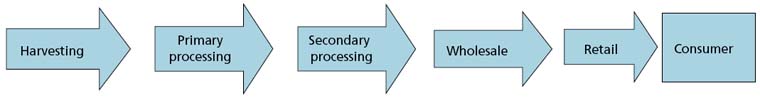
The value chain can be described as the range of activities required to bring a product or service from conception, through the intermediary phases of production to delivery to final consumers (Kaplinsky, 2000). A typical seafood value chain consists of harvesting (either through fishing or aquaculture, or a combination of both), primary processing, secondary processing, distribution and marketing and finally consumption. Figure 6 shows a schematic presentation for typical seafood value chain.
As in other industries there are few, if any, companies which control the whole value chain although concentration within individual segments, or sometimes between levels, has been increasing over the years.
In Figure 6 there are six steps. In reality there could be fewer or more but each step serves as a function which is vital for the entire value chain, i.e. each step adds value to the final product. In traditional business analysis of value chains the focus is on margins or real value added at each level.[12]
Each step in the value chain is analysed in terms of cost items and profit margin. This allows for calculation of the relative weight of each cost item in the overall consumer value.
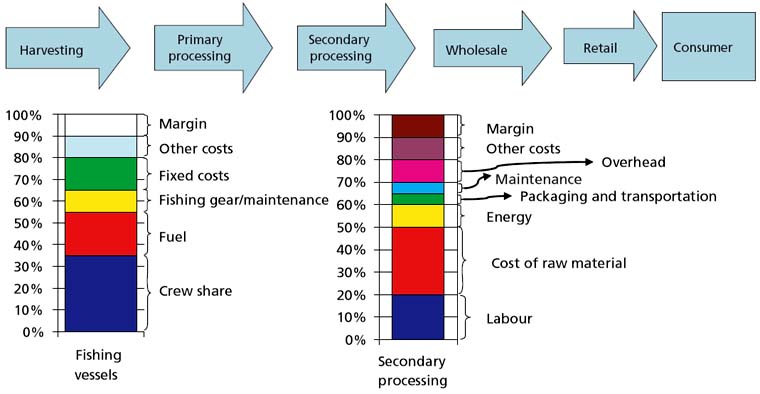
Figure 7 shows an example of the cost items used in the analysis for the harvesting segment and for secondary processing. In order to make the comparison simpler the number of cost items has been kept to a minimum.
Each segment can then be evaluated as a share of the total consumer value. At this step the analysis is similar to analysis which the Economic Research Service of the US Department of Agriculture has conducted for several decades. This allows direct comparison between domestically produced agricultural products and internationally traded seafood products. The comparison is interesting because one would expect significantly different outcomes since the value chain for international trade is considerably longer than for products traded domestically. Vertical integration has also been a major issue in the production and marketing of agricultural products in the US, something which is increasingly seen in the seafood industry. Hence, one could expect that the seafood value chain might develop in similar ways as the US agricultural value chain has over the past two decades.
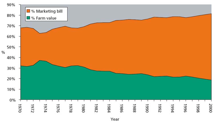
Over the past 30 years there have been substantial changes in the value chains for agricultural products in the United States of America. Figure 8 shows expenditure on food items split between farm value and the marketing bill, measured in constant US dollars. The marketing bill refers to all costs associated with getting the product from the primary producer (in this case the farmer) to final consumption by the customer.
|
FIGURE 7
|
|
FIGURE 8
Source: USDA - Economic Research Unit |
The figure shows that the marketing bill has increased its share from 68 percent of consumer expenditure to 82 percent in 2000. There are several reasons for this increase, most notably higher expenditures on away-from-home food items. Consumers in the United States are buying more food that is prepared away from home, or prepared and consumed away from home. Hence, more non-food resources are needed to provide these services, including labour for services and premises for restaurants. This trend seems to be continuing and as a result the farm value will decrease as a share of consumer expenditure in the near future.
TABLE 4: US farm value share of retail price in 2000
|
Product |
% |
|
Beef, choice, 1 lb. |
49 |
|
Chicken, broiler, 1 lb. |
48 |
|
Pork, 1 lb. |
31 |
|
Peas, 303 can (17 oz.) - canned |
22 |
|
Potatoes, 10 lbs. - fresh |
17 |
|
Chicken dinner, fried, |
14 |
|
Green beans, cut, 1 lb. - frozen |
5 |
|
Tomatoes, whole, 303 can - canned |
7 |
|
Raisins, 15-oz. box |
16 |
|
Flour, wheat, 5 lbs. |
19 |
|
Rice, long grain, 1 lb. |
14 |
|
Potatoes, French fried, frozen, 1 lb. |
10 |
|
Bread, 1 lb. |
5 |
|
Corn flakes, 18-oz. box |
4 |
|
Corn syrup, 16-oz. bottle |
3 |
Source: USDA
The marketing bill is a combination of various activities but the USDA measures the activities by use of inputs rather than as a value chain of activities. In 2000 non-farm labour was the single largest input with 39 percent of the consumer dollar in the US, next was packaging with 8 percent and transportation with 4 percent. Other items include energy, insurance, advertising, interests and profits.
Farm value as a share of retail value varies substantially between food items. Table 4 shows the farm value as a percentage share of the retail value for several common food items.
The table shows that the farmer’s share ranges from 3 percent for corn syrup to 50 percent for beef. At this point it must be emphasized that the share of farm value in the retail price does not say anything about how well individual farmers are doing financially. The economic performance of individual farmers depends on farm related costs, given the revenues for the crop or livestock. Hence a farmer who receives 3 percent of the retail price might do better financially than a farmer who receives 50 percent of the retail price. The table above reveals some additional facts when examined closely. All fresh products receive a higher share of the retail price compared to frozen and canned products. The farmer receives 17 percent of the retail price for fresh potatoes in contrast to 10 percent of the retail value for French fried potatoes. The lower share for the French fries reflects the value added activities in cutting and frying the potatoes for the consumer.
The methodology in this report represents only a snapshot of the distribution of revenues through value chains in order to estimate the share of each market level in the chain. In order to utilize this information to the fullest extent it would be necessary to collect information over a period of time, or at selected points in time, to estimate the changes in the share of each market level when price changes at the consumer level. That type of analysis might yield information about market efficiency and transparency of information between market levels.
An issue that has not been addressed so far is the increasing degree of concentration in the retail sector, particularly in developed economies. In many European countries as well as North America, large supermarket chains have developed rapidly during the last decades and now control as much as 80 percent of retail sales in many markets. This has led to concerns that these outlets are exploiting buyer power (Cooper, 2003). A similar development has also taken place in many processing industries as the efficient scale of operations increase. The same trend has also been seen in the seafood industry. For instance, Murray and Fofana (2002) show that in the UK, the supermarket chains share of seafood sales increased from about 20 percent in the 1980s to over 80 percent in 2000. Little empirical research has been conducted on these issues. However, it is clear that concentration is not necessarily bad. If concentration is due to a technical development where increased scale of operation allows retailing and processing costs to be reduced, making products less expensive for consumers, it improves welfare. Morrison (2001) indicates that this is the case for the concentration in the US meat packing sector. As long as the retail price for the product is reduced, some exercise of market power may also improve welfare. However, excessive market power will reduce value added at other levels in the value chain. The methodology used here does not allow detection of market power, but accumulation of a large share of the retail value of a product at a specific level in the chain compared to similar chains may be an indication of market power being exploited.
Taking these caveats into account four different fisheries in four different countries are examined in order to obtain a snapshot of each market level in the respective fisheries. The fisheries are the Icelandic cod fishery, Tanzanian Nile perch fishery, the Moroccan anchovy fishery and the Danish herring fishery. The Icelandic and Tanzanian fisheries produce fresh and frozen white fish fillets sold in the US and Europe, while the Moroccan and Danish fisheries produce canned and pickled (cured) products from small pelagic species, which are also sold in the US and Europe. The diversity in product form and species makes direct comparison difficult but it gives a broad picture of the complex seafood trade in the world.
|
[3] See e.g. Kurlansky (1997)
for a very entertaining account of the cod trade, which was the major seafood
commodity traded during the middle ages. [4] See Anderson (2003) for a review on the origins and development of seafood trade. [5] Munro (1996) gives a brief account of the development of fisheries regulations and the law of the sea. [6] See DeVoretz and Salvanes (1993), Gordon, Salvanes and Atkins (1993), Gordon and Hannesson (1996), Asche and Sebulonsen (1998) and Asche, Bremnes and Wessells (1999). [7] This is basically the same as assuming that the local agents do not have market power on the world market if they coordinate their actions. [8] The supply schedule needs not be upward sloping if there is increasing returns to scale. However, it is highly unlikely at the production levels where most fisheries operate. [9] See e.g. Krugman and Obstfelder (1994). With well managed fisheries this is also shown more rigorously by Hannesson (1978). [10] See Copes (1970) for detailed analysis of backward bending supply curves. [11] This is just a result of the way that the curves are drawn, although one such point will always exist. [12] For detailed explanations see Shank and Govindarajan (1993) and Porter (1985) |
![]()
![]()
![]()