![]()
![]()
![]()
Figure 15 summarizes the changes occurring on the floodplain throughout one complete floodplain cycle.
The inter-relationships of factors affecting the aquatic phase of the cycle only have been presented by the University of Michigan (1971) (Fig.16). This figure is especially valuable in indicating future lines of research. For a good understanding of the ecology of the floodplain situation many of the interactions shown will have to be quantified.
TABLE XII
Analysis of accuracy of prediction of future catch from regression equations derived from past history of the fishery
| Year | HI | Cest | Actual Catch (C) | Regression | Accuracy of prediction [Cest/C ×100] | ||||
| a | b | r | Sy·x | ||||||
| KAFUE | 1959 | 49.1 | 5 401 | ||||||
| 1960 | 28.6 | 2 983 | -390 | 117.9 | 1.0 | - | - | ||
| 1961 | 22.7 | 2 287 | 4 781 | 2 781 | 48.0 | 0.53 | 1 506 | 48 | |
| 1962 | 41.1 | 4 755 | 4 650 | 2 804 | 46.6 | 0.54 | 1 066 | 102 | |
| 1963 | 69.4 | 6 040 | 8 554 | 1 175 | 97.2 | 0.88 | 1 136 | 71 | |
| 1964 | 83.6 | 9 298 | 9 706 | 997 | 102.2 | 0.94 | 992 | 96 | |
| 1965 | 57.7 | 6 892 | 8 036 | 1 011 | 105.1 | 0.93 | 1 003 | 86 | |
| 1966 | 35.2 | 4 712 | 7 396 | 1 911 | 93.5 | 0.84 | 1 349 | 64 | |
| 1967 | 23.7 | 4 127 | 3 514 | 1 672 | 97.2 | 0.87 | 1 265 | 117 | |
| 1968 | 25.3 | 4 132 | 5 928 | 2 214 | 88.9 | 0.83 | 1 315 | 70 | |
| 1969 | 21.0 | 4 081 | 5 957 | 2 747 | 80.2 | 0.79 | 1 362 | 69 | |
| 1970 | 64.1 | 7 888 | 6 747 | 2 861 | 75.4 | 0.78 | 1 333 | 117 | |
| 1971 | 61.5 | 7 497 | 5 988 | 125 | |||||
| SHIRE | 1969 | 53.5 | 6 944 | ||||||
| 1970 | 25.9 | 8 267 | 9 508 | -47.9 | -1.0 | ||||
| 1971 | 104.0 | 4 523 | 9 039 | 7 241 | 13.8 | 0.51 | 1 284 | 50 | |
| 1972 | 171.5 | 9 603 | 13 062 | 6 036 | 37.1 | 0.9 | 1 404 | 74 | |
| 1973 | 53.8 | 8 032 | 7 551 | 106 | |||||
| NIGER | 1966 | 1 407 | 47 467 | ||||||
| 1967 | 1 211 | 41 985 | 8 114 | 28.0 | 1.0 | ||||
| 1968 | 1 322 | 45 040 | 44 625 | 8 233 | 27.8 | 1.0 | 378 | 101 | |
| 1969 | 1 291 | 44 072 | 45 173 | 9 732 | 26.8 | .97 | 719 | 98 | |
| 1970 | 1 248 | 43 210 | 46 015 | 17 998 | 20.9 | .76 | 1 476 | 94 | |
| 1971 | 1 128 | 41 550 | 36 338 | -2 949 | 36.7 | .88 | 2 099 | 114 | |
| 1972 | 706 | 22 972 | 32 356 | 15 694 | 22.2 | .92 | 2 409 | 71 | |
| 1973 | 562 | 28 152 | 21 172 | 8 339 | 28.0 | .96 | 2 872 | 133 | |
| 1974 | 500 | 22 372 | 14 816 | 151 | |||||
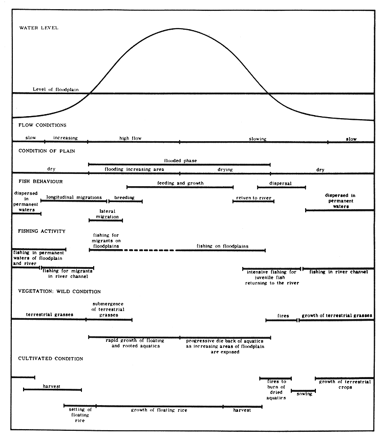
Figure 15 Summary of the major cycles of a floodplain throughout the year
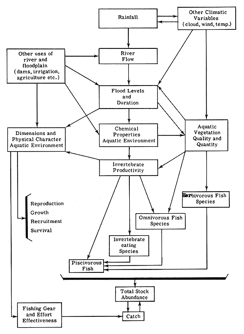
Figure 16 Some interrelationships of factors affecting fish production on floodplains (from University of Michigan, 1971)
Because little research is at present in progress on the fisheries of tropical floodplains, a simple computer model of a floodplain and its fish population has been constructed. This has two purposes. Firstly, to provide qualitative answers to questions on the way floodplain fish populations are likely to behave under different regimes of flooding and exploitation, and secondly to identify areas which need study to give a clearer understanding of the fisheries ecology of such systems.
The model has been constructed from what is known of floodplain fish populations as summarized in this document. Wherever possible actual values for mortality, growth, density of populations, etc., have been employed, but unavoidably certain assumptions have had to be made. The model is so programmed that all parameters can be altered as required.
Specification of the aquatic system: The aquatic system consists of two main elements, the low water system and the floodplain itself. The low water system has two phases. The first from 0–0.69 m depth is described by the formula
Area(ha) = 28 571 water level (m)
and represents a V shaped river channel providing for decreased area and volume with lowered levels. The second, from 0.70–1.00 m has a constant area of 20 000 ha but different volumes at different levels.
Area(ha) = 28 571 water level (m) and represents V shaped river channel providing for decreased area and volume with lowered levels. The second, from 0.70–1.00 m has a constant area of 20 000 ha but different volumes at different levels.
Water level 1.00 m represents the bank-full state.
The floodplain from 1.00 m upward is described by the formula
Area(ha) = 20 000 + 167 672 logℓ water level (m)
Water levels are specified at 52 weekly intervals and enable a number of flood regimes to be described, including different flood/residual water ratios. Flood regimes are specified so that the ascending level crosses 1.00 m at week 1.
An index F is calculated from the sum of weekly water level values from week 1 until maximum level is reached.
The volume of water in the system is computed for each week (x) as xV = xA(xWL)×104.
Sample values of area and volume at different water levels are as follows.
| Level (m) | Area (ha) | Volume (m3) |
| 0.25 | 7 143 | 1.79 × 10⁷ |
| 0.50 | 14 286 | 7.14 × 10⁷ |
| 0.75 | 20 000 | 1.50 × 10⁸ |
| 1.00 | 20 000 | 2.00 × 10⁸ |
| 1.5 | 87 985 | 1.32 × 10⁹ |
| 2.0 | 136 221 | 2.72 × 10⁹ |
| 2.5 | 173 636 | 4.34 × 10⁹ |
| 3.0 | 204 207 | 6.13 × 10⁹ |
The fish population: The fish population consists of a single species stock which grows through five years. The stock may also represent a group of species having similar recruitment, growth and mortality characteristics. Modifications to the number, length and weight of fish in each year class are affected by recruitment, growth and mortality as follows.
Recruitment: The total number of recruits to the stock is determined by the number of fish (n) of age groups II, III, IV and V at week 52 of the preceding year. Recruits to the stock enter at 2 cm length and the recruitment figures include mortalities which have occurred from hatching to this length and are thus not equivalent to known fecundity figures.
An assumed basic number of recruits per individual fish (r) is specified, but this number is adjusted for flood intensity (F) by a factor α, where log10α = 0.58 log10F-0.79. Sample values for recruitment at different flood indices are as follows:
| Age Group | F | ||||
| 3 | 13 | 23 | 33 | 43 | |
| II | 3.07 | 7.18 | 10.00 | 12.32 | 14.37 |
| III | 6.13 | 14.36 | 20.00 | 24.65 | 28.74 |
| IV | 10.73 | 25.13 | 35.00 | 43.13 | 50.29 |
| V | 18.40 | 43.08 | 60.00 | 73.94 | 86.21 |
The recruits are inserted as new age group I and all other age groups move up one, the number of fish in old age group V disappearing.

Although this transfer operation is carried out at week 0 i.e., before any other operations of the current year are affected, recruits (On1) are inserted over a 9 week period according to the following percentages: 50, 20, 10, 8, 5, 3, 2, 1, 1.
Growth: Growth proceeds according to the general formula:
Length at week x for age group y [xly] = KyLogeWkx+52ly-1
where Ky is a growth coefficient characteristic of each age groups, and 52ly-1 is the terminal length of the preceding age group at the end of the previous year. 52ly-1 = 2 cm for fish of age group I. The growth coefficient K is derived from a basic growth coefficient (g) characteristic of each age group: I, g = 3.29; II, g = 2.53; III, g = 1.27; IV, g = 0.76; V, g = 0.51 - which is adjusted for flood intensity F according to the following formula: Ky = gy(0.01F + 0.8). Growth curves of individual age groups in any one year obtained by this means approximate to the known natural condition where about 75 percent of the growth is accomplished by the middle of the floods. Over all growth of one year class through the five years approximates to the classic von Bertelanffy curve. Sample values for terminal lengths of each age group are as follows.
| Age Group Length (cm) | |||||
| Flood Index (F) | I | II | III | IV | V |
| 3 | 11.84 | 20.14 | 24.31 | 26.80 | 28.47 |
| 13 | 14.09 | 23.39 | 28.05 | 30.85 | 32.72 |
| 23 | 15.39 | 25.69 | 30.85 | 33.95 | 36.02 |
| 33 | 16.69 | 27.99 | 33.66 | 37.05 | 39.33 |
| 43 | 17.99 | 30.29 | 36.46 | 40.15 | 42.63 |
Lengths (1) are converted to weights by the generalized formula Wgms = 0.0251 13 giving the following sample weight values:
10 cm = 25.10 g; 15 cm = 84.77 g; 20 cm = 200.95 g; 25 cm = 394.8 g; 30 cm = 678.20 g; 35 cm = 1 076.97 g.
After the weekly growth has been computed the ichthyomass is expressed in terms of weight of fish per unit volume (B) for calculation of mortality coefficients.
Mortality: The number of fish in the system is reduced weekly by applying a density dependend mortality coefficient according to the generalized formula: loge x+1 ny = loge xny - Zy.
The mortality coefficient Z is obtained from a base mortality coefficient z characteristic of each age group which is operated upon by a factor β. The weekly base mortality coefficients are I, z = 0.0453; II, z = 0.0274; III, z = 0.0136; IV, z = 0.0100; V, z = 0.0124, and β is calculated from the formula: logeβ = 1.0238 loge xB - 3.7132 which depends on the density of fish in the system at week x. This expression may be varied so as to simulate systems of different basic productivity. In this model the value of β is 1 when the density of fish is 37.6 g/m2 which is equivalent to a standing stock of 376 kg/ha at a depth of 1 m.
After the above operations are carried out the weekly total ichthyomass and ichthyomass per unit area are available for printout together with water level and length, weight and number of each age group.
The fishery: The effects of fishing may be estimated in a number of ways. By straight removal of a percentage of the ichthyomass, by removal of numbers of fish of any preselected length or age group, or by removal of all fish from a specified area. Removals can be programmed weekly and different types of fishing regime and gear can be simulated.
Figure 17 shows a sample printout from the model with respect to variations in water level and total ichthyomass with time. Further investigations of the effects of changes in hydrological and fishery regimes will be published at a later date together with an evaluation of the model. The present model has its limitations, for instance, present indices do not permit a distinction to be made between the short intense type of flood and the prolonged weak flood (which may give the same index value), thus the effects of duration and intensity as individual components of the flood regime are impossible to assess. In addition to the absolute values of flood height and water retention, the abruptness of change may also influence certain factors. Thus, a slow rise in level at the beginning of the floods is thought to be more favourable to reproductive success than an abrupt rise. Similarly, rapid drawdown, which does not give fish adequate time to leave the plain, would result in increased natural mortality. Unfortunately, however, insufficient information exists to enable an assessment to be made of the relative importance of rate of change on the system. Hastings (pers. comm.) for instance, considers the rate of rise and fall of the water as one of the major factors controlling fish abundance in the Shire system. This view is to a certain extent showed by Lelek and El-Zarka (1973) who attribute changes in species composition in fish populations downstream of the Kainji dam to the effects on reproduction of the sharp changes in water level.
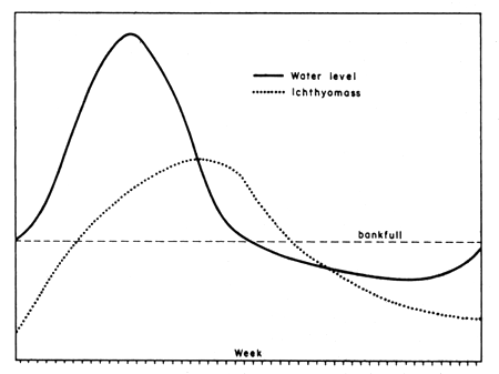
Figure 17 Computer derived plot of water level and ichthyomass in a one year cycle of a theoretical floodplain fish populations
![]()
![]()
![]()