![]()
![]()
![]()
Developed jointly by UNCTAD and FAO, the Agricultural Trade Policy Simulation Model (ATPSM) is a comparative-static, multi-commodity, multi-region, partial-equilibrium global trade model designed primarily for simulating agricultural trade policies, notably in the context of the WTO Agreement on Agriculture[12]. It can simulate the effects of a range of trade policy instruments, notably:
Reduction of out-of-quota (or MFN) tariffs, either by a certain percentage, or with the tariff harmonizing Swiss formula.
Reduction of in-quota tariffs
Expansion of TRQ volumes
Reduction of domestic subsidies
Reduction of export subsidies
The model explicitly covers 161 countries or country groups (the EU-15 is one such country group) and a total of 36 agricultural commodities. It allows users to define groups of countries and commodities, e.g. LDCs or SADC or cereals, and apply different reduction rates (policy reforms) to selected countries and commodities.
The model is calibrated to a base period data set, which describes a world trade equilibrium in some given period. Such a period could be the average of some years. To understand what calibration implies, consider figure 1. To make the graphical illustration empirically meaningful for simulations one has to specify explicitly functions for the demand and supply lines illustrated there. Consider then the specification of the domestic market in country 1. In any given period observed in the real world, the domestic market will equilibrate at some prices such as for instance Pd in figure 1a. In other words we can observe the values of production and demand equal to OA' and OB' in that figure, as well as the equilibrium domestic price and the world price (or the international price plus the domestic-international wedge due to policies). If we know the values of the price elasticities of demand and supply at the relevant price- quantity points on the respective supply and demand curves, then the lines D1 and S1 can be specified completely. Once they are specified for all countries, then the model can be used to simulate alternative equilibria under different policy regimes. This implies that to fully specify the model one needs base period values for all the quantities demanded and supplied by all countries, the values of all policy induced price wedges, as well as the elasticities of supply and demand.
In ATPSM, besides the usual base period quantities and values, all policy instruments are defined in ad-valorem equivalents terms. Thus, specific tariffs are converted to ad valorem rates and both domestic and export subsidies are expressed in their respective ad-valorem equivalents.
The four key variables that are part of an equilibrium accounting relationship are quantities of production, import, export and consumption, with production plus import being equal to consumption plus export. Of these, production and consumption depend on domestic prices. Imports and exports clear the world market. Domestic prices are determined as a function of world market prices and policy variables, e.g. support measures, tariffs, subsidies and quotas. The world prices are linked to domestic prices by price transmission equations that allow world price changes not to be transmitted fully to the domestic market, if that is the reality. In the version of the model utilized here these transmissions are assumed to be complete. As domestic prices are linked to world prices, the basic equilibrium variables are world prices, with domestic prices being determined by the respective policy wedges. Both demand and supply specifications account for substitution effects among commodities.
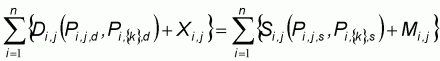
The base period equilibrium of the model can be expressed as follows
|
|
(1) |
|
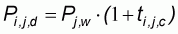
|
(2) |
|
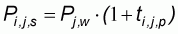
|
(3) |
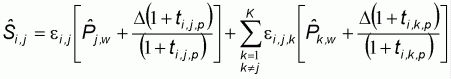
In the above equations, the subscript i denotes the country, the subscripts j and k denote commodities, D(.) and S(.) denote the domestic demand and supply functions respectively for the j'th commodity in country i, M and X denote imports and exports respectively of commodity j in country i, Pi,j,d denotes the domestic demand price of commodity j in country i, Pi,j,s denotes the domestic supply price of commodity j in country i, the group {k} in the subscripts of the second price terms in the demand and supply functions denote the prices of other commodities that substitute or compete for resources for commodity j in country i, n is the total number of countries that produce and trade the commodity in question, the vectors Z and W denote other non-price variables that affect domestic demand and supply of the commodity j in country i respectively, Pj,w is the world price of commodity j, and tc tp denote the consumption and production tariff equivalent wedges between domestic and international prices for commodity j in country i. The endogenous variables are the quantities demanded and supplied, as well as the world prices. Exogenous variables are the demand and supply policy wedges, as well as all other variables that affect supply and demand.
Equation (1) above represents the world equilibrium in the market for commodity j in some period, while equations (2) and (3) summarize the impacts of various policies on domestic consumer and producer prices respectively. Notice that time is not shown in any of the equations. This is because the model is a comparative static one. In other words the model answers the following question. Starting from world equilibrium in a given period, what would this equilibrium have looked like if there were some changes in policy and other exogenous variables in the same period as the base one. In other words the comparative static framework is atemporal, but it is appropriate for analyzing policy questions. Transforming this framework into a predictive one is a much more difficult task, that would entail detailed description of all the dynamic relationships in the market of the commodity.
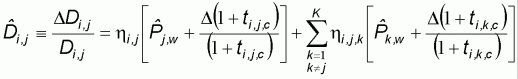
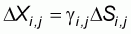
In a fully specified model, the values for all variables in this equilibrium are observed in the base period. A new equilibrium, after some changes in the policy variables can be computed by estimating the proportional (or percentage) changes from the base values of all the endogenous variables of the base equilibrium indicated in (1) as follows (^ denotes a proportional change and D absolute change). Once these percentage changes are estimated, the new level values of all variables can be computed as follows.
Changes in domestic demand for commodity j in country j:
|
|
(4) |
where h denote demand elasticities (own and cross) in country i, and K is the number of other commodities that substitute in consumption,
Changes in domestic supply for commodity j in country i:
|
|
(5) |
where å denote the own and cross elasticities of supply of the j'th commodity in country i. The changes in imports and exports of commodity j in country i are expressed as follows:
|
|
(6) |
|
|
(7) |
where g is the ratio of exports to production (assumed fixed).
There are thus four equations for the changes of the endogenous variables for each country. The export equation implies that that the change in export in each market is some proportion of the change in production. This proportion is estimated by the base year ratio of exports to production, and stays fixed for the simulations.
The solution to the model is obtained by making the sum of all changes in exports of the commodity from all countries, equal to the sum of all changes in imports. It can be easily seen that because of the linearity of the equations in (4)-(7), with respect to the world price changes, the change in the world price can be obtained simply by matrix inversion.
Some of the solutions to the above equation systems are important impact indicators, notably changes in the world prices as well as the volumes of production and exports, following a simulation run. Other indicators follow from these quantity responses, such as DM, DD, and domestic price changes.
The impact on trade revenue following a policy change is computed for each country and commodity, simply as the difference between changes in export earnings and import bills for the commodity in question, namely cotton:
|
Change in export earnings = (Pw1 X1 - Pw0 X0) |
(8) |
|
Change in import costs = (Pw1 M1 - Pw0 M0) |
(9) |
where, the superscripts 0 and 1 indicate base period and simulation values respectively.
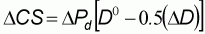
Another key indicator is total welfare and its constituent parts, namely producer and consumer surpluses and government revenue. Total welfare is the sum of the three, DW = DPS + DCS + DNGR[13]. For each country and commodity, changes in producer and consumer surpluses are defined as follows:
|
|
(10) |
|
|
(11) |
where cDU is the change in quota rent received, and thus added to producer surplus.[14]
The change in net government revenue (DNGR), the third term of total welfare, includes changes in various government revenues, notably tariff revenue, export subsidies, domestic support expenditure and change in quota rent not received by exporters. Formally, for each country and commodity, DNGR = DTR - DES - DDS + (1-c) DU, where TR is tariff revenue, ES is export subsidy expenditure, DS is domestic support expenditure and (1-c) DU is change in quota rent forgone.
To sum up, the model generates outputs for the following variables/indicators:
The model is based on data from various sources. Quantities of production, consumption, export and imports (in metric tons) are from the FAO FAOSTAT database (Supply and Utilization Accounts and Trade Domain data). All prices are expressed in United States dollars and are assembled from various sources. The base period for the model is the average of 1996-2000 for production, imports, exports etc. while tariffs and other policy parameters are based on the final year of implementation of the UR AoA (2000 for developed and 2004 for developing countries)[15]. In-quota tariffs, out-quota tariffs and global quotas are from the AMAD[16] database and were aggregated to the ATPSM commodity levels. UNCTAD COMTRADE[17] is the main source for bilateral trade flows while applied tariffs are from the TRAINS[18] database.
Some of the model limitations include the following. All commodities are assumed to be tradable, i.e. domestic prices are determined by world market prices and policy parameters. There is little disagreement that agricultural commodities are tradables. What is an issue and a limitation for the model is that all agricultural commodities are assumed to be homogeneous, namely there is full substitution between imported and domestic products, and among outputs from different sources. The alternative assumption used by some models is the Armington substitution assumption. However, that approach has its limitations as well, in that one would essentially have to assume the substitution elasticities among different sources of imports. For cotton, it appears that the degree of homogeneity of most traded cotton is such as to warrant the perfect substitution assumption.
Note that while the general theoretical framework allows for the presence of other variables in the supply and demand equations, in the actual simulations, it is assumed that only prices influence demand and supply. This maybe a limitation, as the income effects on demand maybe important, particularly for those economies where cotton accounts for a large share of total domestic income.
Although this does not apply for cotton and this study, the following limitation may also be noted for the sake of completeness. An important assumption is that in-quota tariffs are not relevant even where quotas are unfilled. This means that the higher out-quota tariff or the applied rate, whichever is operative (namely lower) in a particular situation, is the key determinant of domestic price. This assumption tends to overstate the benefits of liberalization, as there may be cases where in-quota rates are the relevant determinants of domestic prices.
|
[12] A recent application of
the model in this context is Poonyth and Sharma (2003). [13] A change in net government revenue, DNGR, is measured as within-quota and out-quota tariff revenue less export subsidy and domestic support expenditures and quota-rent foregone. [14] In the version of the model used here, quota rents are ignored, as they are not relevant for cotton. [15] As noted in section 3, this general rule could not be applied to domestic subsidies because of lack of notifications to the WTO for recent years. [16] AMAD: Agricultural Market Access Data Base,http://www.amad.org/files/index.htm [17] COMTRADE: http://unstats.un.org/unsd/comtrade/ [18] TRAINS: http://r0.unctad.org/trains/ |
![]()
![]()
![]()