7. ECONOMIC EVALUATION OF ENERGY PLANTS

7.1 Introduction

A method has been designed to provide engineers with a tool for synthetic evaluation of the competitiveness of a given technology (e.g., a high-efficiency, gas-fed boiler) with respect to a reference plant (e.g., standard gas-fed boiler).
The need for a practical, analytical tool emerged between 1975 and 1980 in developed countries, following increases in the price of fossil fuels and the resultant spread of “energy-saving” technologies. Indeed, numerous innovative energy proposals were made at that time, and this created some confusion.
Consequently, engineers and final users had to be able to analyze the economic soundness of the options being offered to them.

7.2 The Main Aspects of Energy Investments

Economic analysis of energy plants is always based on the comparison of two plant solutions and their satisfaction of a given energy requirement. Therefore, the data necessary concern variations in a number of parameters (investments, maintenance costs, etc.).
Normally, as we switch from an inefficient to a more efficient solution (from an energy standpoint), investment and operating and/or maintenance costs increase (since more efficient solutions are usually more complicated), while the incidence of the energy source decreases. The same thing happens when we switch from a solution employing conventional sources (fossil fuels, electricity from the national grid, etc.) to solutions that make use of renewable sources. This “energy saving trend” is almost always observed.

Example no. 1: the consumption of an electric, thermal-energy generator is certainly higher than that of a solution involving its combination with a solar collector. In the latter case, however, investments are higher, and routine and special maintenance are more expensive (the number of components is larger, and thus inspection requirements and the probability of accidental breakdowns increase).

Example no. 2: the cost of wood is generally lower than that of any liquid or gaseous fossil fuel (needed to produce the same amount of energy). But plants designed to use wood (especially those with high capacities), are sometimes more expensive and difficult to operate (because of the type of feeding, the cleaning necessary, etc.) than plants that employ other types of fuel.
Even when a certain degree of energy coverage must be guaranteed, savings on energy production costs can be obtained:
- by reducing consumption. For example, by switching from a standard electric motor to a high-efficiency motor;
- by completely or partially replacing some of the energy consumed with a source whose cost is zero. For example, use of a wind turbine together with a Diesel generator, employment of solar collectors to reduce the consumption of an electric boiler, etc.;
- replacement of the source used in the standard solution by one which costs less. For example, switching from a Diesel fuel-fed boiler to a coal-fed boiler.
  
  In the first case, the goal is energy savings, in the second it is a reduction in consumption, and in the third it is a reduction in the cost of the source.

7.3 Basis of the Method and Important Concepts

The method is based on pro-rating the cash flow and hence on calculation of the Net Present Value (NPV).
This makes it possible to quantify, in monetary terms, most of the aspects that distinguish the two technologies being compared.

Generally speaking, when an energy requirement must be met (e.g., home heating), the problem concerns evaluation of the profitability of adopting a more expensive, energy-saving technology, as opposed to the reference solution (the example of the high-efficiency and standard gas-fed boilers also applies here). In other words, the main question is: is it worthwhile to make an additional investment in order to later obtain a reduction in operating costs?
An answer can certainly be provided by calculating the NPV.

For this purpose, the following parameters must be estimated for each year of the plant's useful life (Lu):

the gross benefits obtained from the lower cost of the energy produced;
the difference (positive or negative) in routine and special maintenance costs (variation in operating costs);
the algebraic sum of the gross benefits and the increase (or decrease) in operating costs (net annual benefits, NB). On the basis of the established interest rate (i), the annual net benefits are then “shifted” (PNB) to the time of the investment (year zero).
Their sum (TNB), less the increase in the initial investment (δI), gives the NPV, or the monetary gain (or loss) that the technology will provide during its useful life, when compared with the reference technology.

Using the terminology mentioned above, the following is a summary of the procedure:

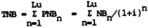
NPV = TNB -δI

The ratio of NPV to the initial increase in investment (δI) is called the profitability index:

Pi = NPV/δI

which is probably easier to use in some situations.

7.4 An Example Applying These Basic Concepts

Let's assume that we have to analyze the profitability of a wood-fed boiler used to heat milk, as compared with similar equipment fed with Diesel fuel. The technical-economic hypotheses contained in Table 3 are assumed to hold true.
The problem is quite simple, since the net benefit is constant throughout all the years of the plant's useful life. The following calculations have to be made:

a) Evaluation of annual savings on energy production (gross benefit):

Where:

HP_w and HP_d are the wood's and Diesel fuel's heat value, respectively;
μ_w and μ_d are the efficiency of the wood-fed and Diesel fuel-fed boilers, respectively;
EC_w and EC_d are the costs of the energy produced with the two fuels, respectively;

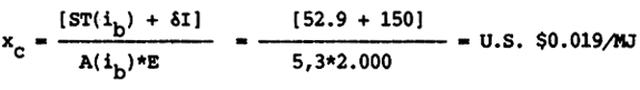
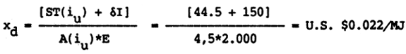
It is observed that (Table 3):

EC_w = biomass cost/(HP_w*μ_w)	= 0.07/(16*0.5) = 0.009 U.S.$/MJ
EC_d = Diesel fuel cost/(HP_d*μ_d)	=0.50/(42*0.7) = 0.017 U.S.$/MJ

Therefore:

Gross benefit (GB) = (EC_d-EC_w)*annual energy requirement =
= (0.017-0.009)*36,000=U.S. $288/year

b) Evaluation of annual operating costs:

It is assumed that analysis of the two plants', maintenance requirements (which are not discussed here, in order not to complicate presentation of the economic concepts) would lead to the following conclusions:

zero costs of labor needed to load the wood and for routine maintenance of the Diesel fuel-fed boiler (family-run plants);
annual visit by an engineer to check on plant operation.

Related costs are estimated at U.S. $80 and $50 (two hours of work and various materials), for the wood-fed and Diesel oil-fed boilers, respectively.
Consequently, the increase in operating costs of a Diesel fuel-fed boiler, as opposed to a wood-fed model, is U.S. $30/year (this value does not change throughout the plant's useful life).

c) Evaluation of the net annual benefits:

During every year “n” of the plant's useful life:

NB_n = Gross Benefit (GB) - annual operating costs = = 288 - 30 = U.S. $258/year

d) Calculation of NPV:

All the annual net benefits are updated to year “O” (i.e., the time at which the investment is made). In other words, the following calculation should be made for each year of the plant's useful life (considering an interest rate of 15% by way of example):

PNB_n = NB_n/(1+i)ⁿ

Thus, for the first year:

PNB₁ = 258/(1+0.15)¹ = U.S. $224.30

whereas, for the fifth year:

PNB₅ = 258/(1+0.15)⁵ = U.S. $128.30

It can be observed that the present value of the benefits decreases as n increases. In other words, future savings are worth “less” at the time when the cash outlay is made than short-term savings.
The results of each individual operation are then added together to obtain the TNB. In this specific case, all the NBs are the same throughout the plant's useful life. Therefore (see Table 4, initial summation), TNB can be calculated by the following expression:

TNB = [(1+i)^Lu-1]*NB/(i*(1+i)^Lu) = [(1.15)¹⁰-1]*258/(0.15*1.15¹⁰) =
= U.S. $1,295

This figure is the “value” at year “O” of the total savings (which are actually distributed over the course of the useful life).
Finally, if we consider that the additional investment (δI) to switch from a Diesel fuel-fed to a wood-fed boiler is U.S. $1,500:

NPV = TNB - δI = 1,295 - 1,100 = U.S. $195

In other words, NPV represents what's “left in the user's pocket” when he switches from the reference solution to the solution under consideration here.

e) Evaluation of the profitability index:

Pi = NPV/δI = 195/1,100 = 0.18 (18%)

The economic performance of the wood-fed boiler can be considered satisfactory (although, this is still a subjective judgment).

7.5 Comments on the Basic Procedure

The method requires estimation of numerous technical and economic parameters (e.g., the useful life of the plants, their average efficiencies, the users' energy requirements, the maintenance schedule, the duration of components that have to be replaced during the plants' useful life, etc.). Naturally, the reliability of the analysis largely depends on the reliability of the estimates. Therefore, the analyst must have considerable experience with the plants under examination. The problem becomes particularly complicated when innovative or experimental plants are considered, since all the necessary data cannot always be found.
Uncertainties of the data can be lessened by calculating NPV and Pi in relation to their maximum and minimum values (obviously estimated). This provides a measure of the sensitivity of the economic results to the parameters under consideration.

For example, let's assume that we are not sure whether to estimate the annual number of hours required for a given plant's routine maintenance at 50 or 100 hours. The use of an average value (75) is the most logical solution, but doubts remain about the reliability of this evaluation. Indeed, the effect produced by uncertainty becomes immediately apparent if we calculate NPV using the highest and lowest values (100 and 50). When the results obtained differ only slightly, the average value can be readily accepted. But when this is not the case, the problem has to be analyzed more deeply (by referring to specific documentation, consultants, etc.).
In order for the proposed plant to be preferable to the standard version, its NPV (and hence its Pi) must be positive. This is a necessary, but insufficient, condition. In some cases, for example, the user may feel that the NPV (or Pi) calculated does not justify the inevitable risks that go hand-in-hand with more complex plants (e.g., a Pi of 10% may be considered too low);
The user is sometimes forced to reject sound operative proposals because he cannot come up with the required capital. For example, let's assume that a complete overhaul of the energy plants at a milk processing center would reduce consumption by 50% and that Pi is estimated at 30% (based on improved product quality, as well), but the capital required is U.S. $2,000. This figure may be prohibitively high if it is impossible to get a mortgage, negotiate extensions on payments, etc. Therefore, plant solutions requiring lower investments are naturally more competitive (even when these plants save less energy);
More complex cases have to be analyzed carefully. For example, when evaluating gross revenue, the profits deriving from the use or sale of the following products can sometimes be added to the benefits provided by energy savings:
- byproducts of the proposed technology (e.g., the ash produced by the combustion of husks, the increased nitrogen content of sewage treated in anaerobic fermentation plants, etc.);
- surplus energy (e.g., an electric generator that supplies part of its energy to another user).

In highly complicated analyses, values of NB can vary from one year to the next because of the company's production schedule, presumed price variations over time, etc.

7.6 The Complete Method

NPV and Pi are closely connected with the net price of the energy saved or replaced (P_s) and the interest rate adopted, i. Therefore, analysis of the sensitivity of these values to the two parameters will show:

the influence of variations in the price of the energy source employed by the reference plant (usually a fossil fuel);
the “critical” prices of the source at which the technologies are or are not profitable;
the influence of financial limitations (generally linked to i).

For example, the following equation shows how Pi is connected with the price of the replaced source:

Pi = a + b*p_s

where a and b are constants that depend on the plant's technical and economic characteristics. The connection between Pi and P_s is linear.
If, in addition to P_s, the rate of interest i also varies, a sheaf of straight lines passing through a set of coordinates (x_a, -1) is plotted on a cartesian plane P_s -Pi.
In practical terms, it is useful to consider a sheaf formed by three straight lines calculated using the following rates (Figure 5):

i=O;
i=the cost of money (i_b, that is, the rate on bank loans);
i=interest desired by the user (i_u, that is, the rate of return on capital that would make the investment attractive to the user).

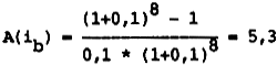
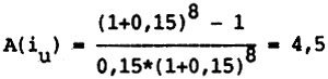
In principle, i_u>i_b, since it is assumed that the user is only interested in a plant whose yield is higher than the interest rate to be paid to third parties for loans.
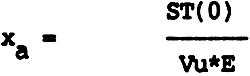
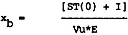
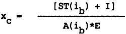
On the abscissa (i.e., Pi=0 or NPV=0, which is implicit), the three lines identify four energy prices (x_a, x_b, x_c and x_d) to which particular conditions correspond.

In fact, when:

P_s = x_a:	the proposed plant's annual net benefits equal the variations in operating costs: in other words, the annual net benefits are always zero;
P_s = x_b:	over the course of the plant's useful life, the annual net benefits are able to “cover” (at an interest rate of zero) the additional investment; in other words, this is the payback price, where the payback period is equal to the presumed life of the plant;
P_s = x_c:	there is no difference between the reference and the proposed solution from an economic standpoint;
P_s = x_d:	the proposed solution makes sense for the user, since the plant returns i_u, with respect to the reference solution.

The method is simple to use: equations for three straight lines on the plane P_s-Pi are determined (e.g., by calculating two values of Pi for each line in correspondence with two prices P_s) for a given combination (consisting of the reference plant and the proposed plant).
Once the graph has been completed, the current price P_a of the energy saved or replaced is located with respect to prices x_a, x_b, x_c and x_d.

Five situations are possible:

P_a<x_a:	the proposed technology is not economical at all, since its operating costs are higher than its gross benefits (Pi<-1; Figure 6);
x_a<P_a<x_b:	annual balances are positive, but not sufficient to guarantee a full return on the capital invested (even when i=0; Figure 7);
x_b<P_a<x_c:	the capital has not yet been recovered (indeed, Pv<0; Figure 8);
x_c<P_a<x_d:	the economic balance is positive, but lower than that desired by the user (Figure 9);
P_a>x_d:	economic performance is equal to or higher than the minimum desired by the user (Figure 10).

In conclusion, the graph can be used to evaluate the “°” of profitability of the proposed solution in comparison to the reference solution.
If we assume that the gross benefits are constant throughout the plant's useful life Lu (which is almost always the case), the values of x_a, x_b, x_c and x_d can be supplied by the following equations:

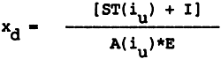
Where:

E is the energy saved (net) when the goal is energy savings or decreases in consumption, whereas it is the user's thermal requirement in the case of reduced source costs.
ST(x) is the variation in routine and special maintenance costs, pro-rated at rate x, when the goal is energy savings or decreases in consumption; it is the variation in maintenance costs (routine and special) plus the costs relating to the supply of energy for the proposed solution (pro-rated at rate x), in the case of reduced source costs.

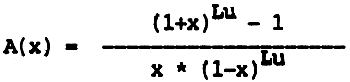
A(x) is a financial operator defined by the equation:

When difficulties connected with estimation of the various parameters (see points a and b in section 7.2) can be overcome, application of this method is fairly rapid.
In fact, once values have been determined for the four points, the three straight lines can be traced and a final judgment can be made.

Calculation of ST(x) can be difficult in more complicated cases and when manual methods are used. However, this problem can be solved by using work sheets and programmable calculators (even those with few functions). Standard programs, which make rapid calculation possible, are available for these machines.

7.7 Additional Information Provided by This Method

An economic index that is frequently used is the internal rate of return (IRR). This index is, by definition, the rate of interest that reduces NPV to zero. With reference to the terminology used above:

TNB(IRR) - δI = 0

Calculation of NPV and IRR gives a fairly precise idea of the economic performance of an investment. The former value provides the amount of savings obtained and the latter the rate of interest that would make the reference and proposed plants economically equivalent.
Consequently, the information obtained may be considered complementary.

IRR is usually determined through iterative calculations. The rate of interest is varied until NPV=0. Therefore, this procedure requires the use of a computer.
The proposed method provides an approximate evaluation of IRR, which is sufficient to reach some initial conclusions.
Indeed, in correspondence with points x_b, x_c and x_d, Pv is zero and hence NPV=0.

Thus, it is clear that:

for P_a=x_b	→	IRR=0;
for P_a=x_c	→	IRR=i_b;
for P_a=x_d	→	IRR=i_u;

and

for P_a<x_b	→	IRR<0;
for x_b<P_a<x_c	→	0<IRR<i_b;
for x_c<P_a<x_d	→	i_b<IRR<i_b;
for P_a>x_d	→	IRR>i_u.

By comparing P_a with the values of x_b, x_c and x_d, the corresponding value of IRR can be estimated.

7.8 An Applicative Example

Phase 1: Definition of the problem. The advisability of installing a solar water collector on a 30-m² surface to be used by a milk processing center (for washing containers) to limit the consumption of Diesel fuel by an existing boiler equipped with storage.

Phase 2: Definition of the reference and proposed plants. The reference plant consists of a Diesel fuel-fed boiler; the proposed plant is a combination of this boiler and the solar collector. The goal is a reduction in consumption (solar energy, whose source costs nothing, is employed so as to limit the consumption of Diesel fuel).

Phase 3: Estimation of technical and economic parameters. The increased investment concerns installation of the solar plant; the proposed plant also requires additional maintenance. An initial analysis of the two plants demonstrates the following:

net energy contribution of the solar plant: 2,000 MJ/year per m² of collector;
investment required for the solar portion alone: U.S. $150/m²;
the useful life of the plants: 8 years;
annual routine maintenance costs for the solar section (including the costs of electric energy for circulation of fluid in the collector): U.S. $8/m². During the fourth year, the plastic cover has to be replaced (special maintenance), and the cost of this operation is U.S. $15/m²;
cost of Diesel fuel: U.S. $0.50/kg (heating power: 42 MJ);
average boiler efficiency: 0.6;
interest rates under consideration: i_b=10; i_u=15%.

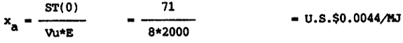
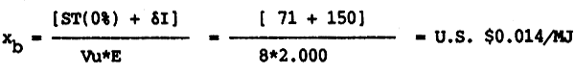
In conclusion, it must be determined whether an investment of U.S. $150 (for simplicity's sake, reference is made to unit of surface area) is justified to obtain an energy savings of 2,000 MJ.

Phase 4: Determination of routine and special maintenance. Let's assume that the gross benefit is constant throughout the plant's useful life (which is an essential hypothesis for application of the calculation formulas). In addition, since the goal here is a reduction in consumption, it is necessary to calculate the discounted values of the costs of routine and special maintenance.

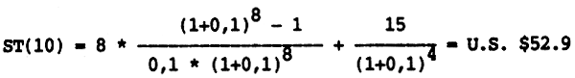
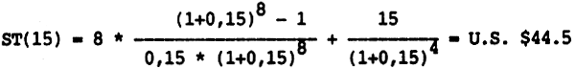
Annual maint. costs (years: 1, 2, 3, 5, 6, 7, 8)	= U.S. $ 8/m²
Annual maint. costs (year: 4) = 8 + 15	= U.S. $23/m²

Discounting these costs at an interest rate of 0% coincides with their algebraic sum. That is:

ST(0) = 8 * 7 + 15 = U.S. $71/m²

For rates of 10 and 15%, however:

Phase 5: Plotting the graph.
Calculation of characteristic points:
for the various rates (0, 10 and 15%):

Since we are concerned with a reduction in consumption, E represents the energy supplied by the solar plant (energy saved).
At this point, the characteristic points can be plotted on the graph, and the three straight lines can be traced.
In our specific case, all the lines will pass through the same coordinates (0.0044, -1), with each one passing through the points (0.014, 0), (0.019, 0) and (0.022, 0).

Phase 6: Reaching a final conclusion. The current cost of energy is equal to:

P_a = (0.5/kg)/(42 MJ/kg^*0.6) = U.S. $0.02/MJ

Then P_a is located between points c and d.

Thus, it is clear that although the proposal is economically profitable, it does not fully meet our expectations.
IRR, which falls somewhere between 10 and 15%, is positive.
To improve the situation, the proposal would have to be revised in order to obtain:

an increase in the plant's useful life;
an increase in the amount of energy saved;
a reduction in operating and investment costs.

7.9 Application of the Method to Feasibility Studies

When an operative hypothesis and an element for comparison exist, this method may be useful for an initial evaluation of a proposal's level of competitiveness, which may be defined as good, improvable or non-existent depending on the situation.
The level of competitiveness may be defined as good (Figure 10) when the current price P_a of the energy that is replaced or saved is higher than x_d. As we noted above, under these conditions the alternative proposal guarantees better results than those desired by the user.
The level of competitiveness becomes improvable when P_a is between x_b and x_d. In this case, economic performance is modest and does not meet the user's expectations. However, revision of the proposal may provide a result that can be classified as “good”.
Finally, the level of competitiveness is defined as non-existent when P_a is lower than x_b.
When P_a<x_a, economic performance is extremely negative.

7.10 Application of the Method in the Study of Financial Subsidies

The “design” or analysis of various forms of assistance is often under consideration to encourage the spread of technologies that are felt to be highly sound for different reasons. In this context, the three levels of competitiveness described above may be interpreted as follows:

Level of competitiveness - Good: the final user already considers the seconomic performance satisfactory, and assistance is not necessary. Consequently, activity can concentrate on the spread of these technologies and various forms of monetary assistance.

Level of competitiveness - Improvable: modest economic performance justifies an analysis of subsidies that could make these technologies more acceptable to the user. The objective should be to encourage the moderate spread of these technologies in order to examine all their technical and economic aspects. In the most unfavorable cases (x_b<P_a<x_c), the possibility of financing exemplary plants (together with research institutes) may be considered.

Level of competitiveness - Non-existent: there is no reason to encourage the spread of these technologies (especially when P_a<x_a). These technologies require further research aimed at increasing their level of competitiveness. Exemplary plants would only be useful in certain cases (when P_a approaches x_b).

References: [6], [7], [8].

Table 3 - Technical and economic data used in comparison of a manual, woodfed boiler (proposed plant) and a standard Diesel fuel-fed boiler (reference plant; see text).

Parameter	Wood-fed	Diesel fuel-fed
Thermal power (kw)	40	40
Energy requirement (MJ/Y)	36000	36000
Investment (U.S. $)	3100	2000
Maintenance cost ($/year)	80	50
Interest rate (%)	15	15
Useful life (years)	10	10
Avg. fuel efficiency (%)	50	70
Fuel's heat value (MJ/kg)	16	42
Fuel cost ($/kg)	0.07	0.5

Table 4 - Useful Financial Formulas

Purpose of the Formula	Equation [1]
shift from year “n” to year “O”	S/(1+i)ⁿ
shift from year “O” to year “n”	S*(1+i)ⁿ
initial accrual of constant annuities (for N years)	A[(1+i)^N-1]/[i(1+i)^N]
Final accrual (during year “N”) of constant annuities	A*[(1+i)^N-1]/i

[1] All the equations refer to deferred annuities (i.e., available at the end of each year taken into consideration, which is usually the actual case).

Terminology: S - sum of money; A- annual share; i - interest rate; n -year between O and N; N - number of years taken into consideration.

Table 5 - List of Symbols Used in the Text

Parameter	Symbol
Net annual benefits during year n (U.S. $)	NB_n
Pro-rated net annual benefits during year n (U.S. $)	PNB_n
Financial operator to accrue at rate x (-)	A(x)
Energy saved or energy requirement (MJ/year)	E [1]
Investment (U.S. $)	I
Profitability index	P_i
Price of energy saved or replaced (U.S. $/MJ)	P_s
Current price of energy saved or replaced (U.S. $/MJ)	P_a
Generic interest rate (%)	i
Bank interest rate (%)	i_b
Interest rate desired by investor (%)	i_u
Operating costs for year n discounted at rate x (U.S. $)	SA_n(x) [2]
Summation of all the SA_n(x)	ST(x) [2]
Internal Rate of Return	IRR
Net Present Value (U.S. $)	NPV
Plant's Useful Life (years)	L_u

[1] E represents the energy saved when the goal is energy savings or a reduction in consumption; it represents the energy requirement when a reduction in source costs is desired (see section 7.6).
[2] Operating costs also include energy costs only when a reduction in the cost of the source is desired (see section 7.6).

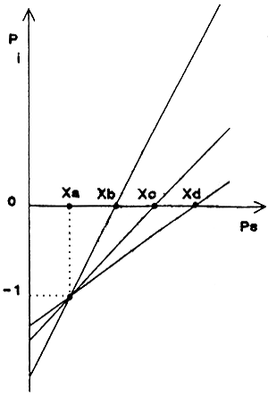
Figure 5 - Profitability index Pi (ratio of NPV to the increase in the initial investment) versus the price P_s of the energy saved or replaced. The three lines are related to the following interest rates: i=0; i=cost of money (i_b; i.e., bank rate on loans); i=the interest desired by the user (i_u; i.e., the rate of return on the capital that would make the investment attractive). The three lines define the points x_a, x_b, x_c and x_d, which are described in the text.

Figure 6 - When the price (or the variation in prices) of the energy saved or replaced (P_a) is less than x_a, the technology is not economical from any standpoint, since the annual net benefits are always negative (costs > benefits). In this case, the degree of competitiveness is non-existent.

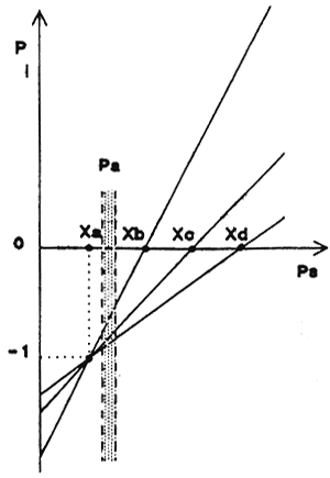
Figure 7 - When the price (or the variation in prices) of the energy saved or replaced (P_a) is between x_a and x_b, the technology is not economical, since the annual net benefits are positive but do not compensate (even with an interest rate of zero) for the initial investments. As in the case in Figure 6, the degree of competitiveness is non-existent.

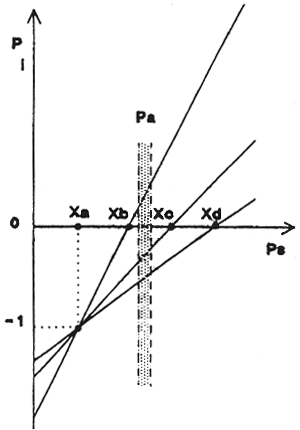
Figure 8 - When price P_a is between x_c and x_b, the technology is only economical when the interest rate is zero. This type of situation is defined as “improvable”, since revision of the project may improve its economic performance.

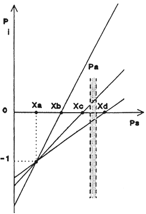
Figure 9 - When price P_a is between x_d and x_c, the technology is economical. Indeed, the initial investment is recovered even when the bank's interest rate is used. However, the user does not consider overall performance adequate (i.e., he feels that it does not compensate for the risks inherent in the proposed technology). As in Figure 8, this situation is defined as “improvable” in terms of economic competitiveness.

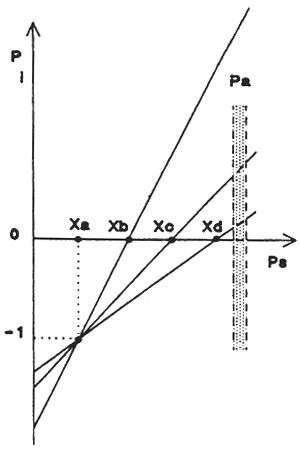
Figure 10 - When P_a is greater than x_d, the technology is economical and profitable. The level of competitiveness is good.