![]()
![]()
![]()
The richness and variety of riverine habitats provide a wide range of possible food organisms and substrates. These originate either from within the aquatic system itself (autochthonous food sources) or from outside the system (allochthonous food sources), although they are all ultimately dependent on materials of external origin in the form of alluvial silt, dissolved nutrients, material washed into the system with surface flow or decomposition products on inundated ground. These nutrients form the basis for numerous sources of food as follows:
| Autochthonous | |
| Plankton community | - phytoplankton |
| - zooplankton | |
| - drift organisms | |
| Benthic community | - mud and associated microorganisms, |
| - coarse detritus, decomposing vegetable or animal remains | |
| - insects and small crustacea | |
| Plant community | - plants including filamentous algae and submersed, floating or emergent higher vegetation |
| Epilithic - Epiphylic | - epiphytic or epilithic algae |
| community (“Aufwuchs”) | - associated microorganisms, insects, crustacea, etc. |
| - this category can include the root flora and fauna of floating vegetation as well as some detrital aggregate, that slimy coating found on submerged parts of plants or rocks which consists of detritus, bacteria and algae. | |
| Neuston community | - surface living insects and larvae at the air/water interface |
| Fish | - including eggs, larvae and juveniles |
| Other vertebrates | - amphibia, reptiles, birds or small aquatic mammals |
| Allochthonous | |
| Vegetable matter | - leaves, roots, flowers, fruit and seeds of plants growing near the water or overhanging the water course which contribute to the surface drift and to the detritus |
| Animal matter | - insects, arachnids, worms, etc., falling on to or washed into the water from terrestrial environment |
In rivers primary production is located more in the proliferation of higher plants than in the phytoplankton. Epiphytic or epilithic algae are abundant only at the fringes of the vegetation mass or on rocks and other supports. Higher plants are themselves useful for food only when young and tender, although fruit and seeds do figure in the diet of some species. The major contribution of higher plants to the nutrient flow is by decay and the consequent enrichment of the detritus. Because acceptable primary plant foods are not common in river floodplain habitats, purely herbivorous species are relatively rare. Species that do eat higher plants or phytoplankton usually have an alternative source of food. In the case of higher plant browsers such as Tilapia zillii, the fish often have recourse to vegetable detritus for the consumption of which they are equally well-adapted. The scarcity of phytoplankton in flowing water systems means that this source of food, so common in lakes, is also of minor importance.
The general absence of primary feeders means that other types of food dominate in the diet of riverine species. Four categories emerge as of particular importance depending on locality within the river system. These are:
Benthos which is particularly important in the headwater streams or in rejuvenated reaches. Benthic organisms are particularly abundant in the rocky and often torrential low order streams but decline in abundance downstream until, in the mesopotamon, they form a relatively minor part of the diet. Thus food supply in such reaches tends to alternate between a variety of forms living in the bottom, usually in the interstices of the rocks, in the riffles, and a drift of such autochthonous benthic organisms and of allochthonous material in the pools. The supply of microbenthos in these spaces between the rocks favours small size thus the young of many species of fish pass the earlier stages of their development within the riffles.
Mud and detritus: Bottom deposits really represent two rather different kinds of food. The detritus feeders rely on coarser decomposing plant material together with associated micro organisms and animal communities. These comprise a high proportion of species particularly in headwater stream and forested habitats where leaf fall accumulates in the slack of the pools or close to floating vegetation where litter is also abundant. The resulting coarse detritus tends to be a feature of low order streams and it becomes finer with progress downstream until, in the potamon, it forms fine organic mud.
Mud itself contains amino acids and other organic products of decay which can be used by fish in combination with the saprophytic bacterial and protozoan microorganisms. Bakare (1970) has analysed this element of the diet of Citharinus and Labeo in the Niger river. The finer the particle the greater its alimentary value, and the preferred particle size was between 0.10 and 0.05 mm, although grains as large as 0.18 mm were taken. The finer fractions contained relatively larger amounts of carbon and nitrogen than did the larger particles. The size of particle and the food content of the deposit, which the fish seemed able to detect, appeared to be the major factors limiting the distribution of these species. At the time of sampling about 70 percent of the bottom deposits were suitable for food. Bakare noted that bottom deposits became progressively depleted of C and N during the flood when C. citharus was actively feeding. Periodic drying of the mud may recharge the organic content through the incorporation of dung and other decaying animal and vegetable matter. Similarly studies by Quiros et al. (1981) in the artificial lake of Salto Grande, a river type reservoir on the Uruguay river, showed strong correlations between both the total organic matter and organic nitrogen concentrations in different locations throughout the lake and the catch of such iliophagous and detritophagous species as Prochilodus platensis, Pseudocurimata gilberti, P. nitens, Curimatorbis planatus, as well as Plecostomus and Loricaria anus. Further evidence for the ability of certain species of fish to feed on amino acids present in bottom mud was produced by Bowen (1980) who found that the substances were readily absorbed along the intestine of Oreochromis mossambicus living in Lake Valencia, Venezuela. Unusual gastric juices are required to liberate protein from this form of detritus and O. mossambicus is recorded as having gastric acid at an uncommonly low pH (<1.5) for fish (Bowen, 1981). Bowen (1979a) had earlier established that benthic detrital-aggregate contained rich organic residues (up to 45.7% carbohydrate and 1.8–14.2% protein) a large proportion of which was in the form of non living amorphous material. Both Bakare and Sandon and Tayib (1953) found a high proportion of mud feeders in the fish populations of the Niger and Nile rivers. In the Niger 10 percent of the species feed exclusively on this source of food and 10 percent more include it as a major element of the diet. The number of species, however, is little guide to the true abundance of mud-eating fish. In the La Plata system, for instance, 60 percent of the ichthyomass of the floodplain pools is located in the main mud-eating (iliophagus) species Prochilodus platensis (Bonetto, Dioni and Pignalberi, 1969). Fish of the genus Prochilodus are widespread mud-eaters in Latin America and are met in equal abundance in other systems such as the Mogi Guassu (Godoy, 1975) and the Magdalena (Kapetsky et al., 1976). Goulding (1980) also confirms that mud and detritus eating fishes of the genus Prochilodus, Semaprochilodus and Curimatus account for a large part of the biomass in the nutrient poor forested floodplains of the Amazonian rivers he studied.
Allochthonous material: Many workers here have remarked on the quantity of allochthonous material consumed by fish in river systems. Not only is such external material one of the two major food sources in headwater streams but on forested blackwater river floodplains the rain of animal and vegetable matter from the overhanging vegetation is the only appreciable source of food and all food chains start from it. Typical of the latter are the Amazon and Zaire rivers from which Geisler et al., (1973), Roberts (1973) and Goulding (1980 and 1981) have noted that food from terrestrial sources is particularly important. Similar observations have been made in the Mekong basin especially in the flooded forest surrounding the Grand Lac. Most species in these habitats show great flexibility in the type of allochthonous food taken, but some fish, such as the frugivores of tropical forest rivers have specialized in using particular food items. Indeed the most exhaustive study carried out on such species (Goulding, 1980) indicates that some Amazonian species of Characidae, Cynodontidae, Anostomidae, Pimelodidae, Doradidae and Auchenipteridae specialize in fruit or seed eating in the Amazon during high water to the extent that over 87% of the total food consumed by Colossoma, Mylosoma, Myleus and Brycon in the wet season was fruit or seeds. The various species even show preferences for particular types of fruit or seed correlated with their dentition. Most such species either cease feeding during the dry season or turn to alternative food sources which in many cases may consist of other allochthonous material such as leaves or flowers, but may as in the case of the piranhas be of living animal origin. The frugivorous habit has been described, or hinted at, by workers from other forested areas. Fruit, seeds and flowers form a component of the diet of Notopterus notopterus, Paralaubuca typus and Clarias batrachus in the Mekong (Bardach, 1959); Distichodus atroventralis and D. sexfasciatus of the Zaire (Matthes, 1964); Leptobarbus melanotaenia, Puntius bulu, P. binotatus, P. bramoides, P. sealei, Botrachocephalus mino and Chonerhinus modestus of North Borneo (Inger and Chin, 1962); Leptobarbus hoeveni of Sumatra (Vaas et al., 1953). Tan (1980) records Tor tambroides, Acrossocheilus hexagonolepis, Leptobarbus hoeveni, Puntus bulu and P. daruphani as gathering around Ficus variegata, Eugenia sp., Diptocarpus oblongifolius, Dypoxylon angustifolium and Elateriospermus tapus to eat the ripe fruit as it falls into the water. Other species have become adapted to taking organisms from outside the aquatic system, the most extreme example of this being found in the Archer fish (Toxotes) which shoots water droplets at insects which settle on overhanging vegetation so as to knock them into the water. Fittkau (1973) has illustrated the type of simplified nutrient-food-consumer cycles that are found in the mouth lakes of the Amazonian tributaries (Fig. 6.1). The role of food coming from outside the aquatic system is not confined to forested rivers, as some species inhabiting savanna plains also rely heavily on this source (Kelley in FAO/UN, 1968a). Adaptations to this are such that Brycinus spp. have been recorded as deliberately jumping against the stems of rice plants to bring down seeds for consumption (Matthes, 1977).
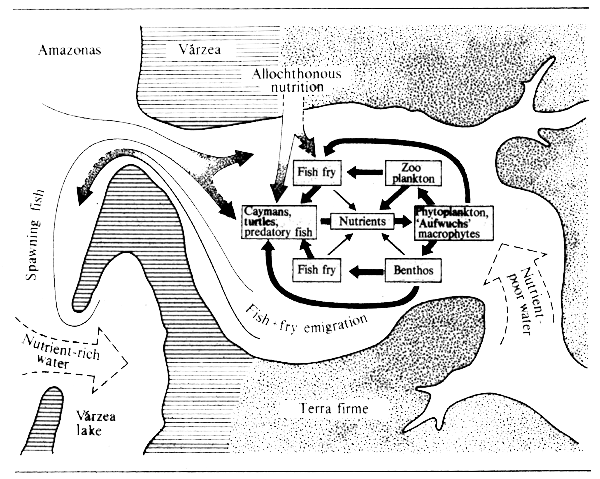
Figure 6.1 The nutrient cycle in the mouthlake of an Amazonian tributary. (After Fittkau, 1973)
Predation on fish and large invertebrates by other fish is relatively unimportant in small streams. Indeed the smaller and more unstable a water course, the less likelyhood that predation will significantly affect its population structure. (Moyle and Li, 1979). In some small coldwater streams more stable conditions allow predation by fish such as trout to play a more significant role. Trout for instance accounted for 15% of the total mortality of other fish in the water course studies by Alexander (1979). The relative importance of predatory species tends to increase downstream until the point where Bayley (1983) found piscivorous predation to account for most of the productivity of small and medium sized fishes in the forestal Amazon. On savanna floodplains there is a tendency for bottom-feeding forms to dominate by weight, although there are usually only a few species at this trophic level. Furthermore in some systems decapod Crustacea perform the primary scavenging role and fish are confined to the higher links of the food chain. In the Potamon community structures usually contain a very high proportion of predatory species and piscivorous predators are generally very common. The relative abundance of these elements of the community tends to increase during the dry season giving the very high predator-forage fish ratio recorded by some authors. For example, Mago-Leccia (1970) noted that up to 75 percent of the population of some floodplain pools of the Orinoco consisted of fish eaters such as Hoplias malabaricus. Lowe-McConnell (1964) and Bonetto, Dioni and Pignalberi (1969) equally commented on the abundance of piscivores and the absence of small fish in flood pools of the Rupununi and Parana rivers respectively at the end of the dry period. I have observed the same phenomenon in the Oueme river and a number of other workers have commented on it in passing with reference to other African systems. Strangely, prolonged and stabilized high water in the normally fluctuating Everglade marshes also produced an increase in predatory species according to Kushlan (1976). This change was due to the migration into the marsh of large predatory species which are normally intolerant of the extreme swamp conditions. Similar shifts may be anticipated where floodplains are impounded to increase the inundation time.
Lowe-McConnell (1975) concluded that there is a linear succession of dominant food sources in streams and rivers. Fishes in headwater streams depend mostly on allochthonous foods. As the stream enlarges grazers and generalized predators feeding on benthic invertebrates become more important. Finally in the lower reaches, the accumulation of detritus and soft mud supports a number of mud-eating species although piscivorous predators are also abundant. Nikolsky (1937) described this same succession from the Amu Darya and Syr Darya and correlated with it the increase in length and complexity of the guts of fish as one proceeds downstream in these rivers. This progression of feeding types is in accordance with the predictions of the river continuum concept and also agrees with similar progressions in other organisms.
Feeding habits of individual fish species in rivers have been described by many authors. These have generally been analysed as trophic “statics” which, by approaching diet in a manner limited in space or time, tends to assign fish to trophic categories or niches. This has led to the assumption that the considerable specializations of dentition, jaw structure, body form and alimentary tract, corresponds to real feeding niches particular to the species. Closer examination of this assumption shows the situation to be considerably more complex. In stable systems such as reservoir rivers it may be supposed that specialization leads to the species adopting a fixed position in the community whereas in fluctuating systems typified by flood rivers specializations may be more valuable in one or other of the phases of the system. There has been some debate as to whether the advantage accrues during times of abundance (usually high water) when adequate food of diverse nature is present or at times of scarcity when specialization would sharpen the competitive capacity for those resources which are available. In support of the latter hypothesis Zaret and Rand (1971) found trophic overlaps in a Panamanian stream to be minimal during the dry season, when food abundance was at its lowest. For example, Astyanax, which normally occupies the surface during the nutrient rich wet season, is forced into the mid waters by the more specialized Gephyrocharax during the dry season. Here access to its usual diet is prevented by Roeboides and as a consequence switches from its normal concentration on allochthonous insects to a purely vegetarian diet. In more temperate waters, Angermeier (1982) also found an increase in the variety of prey selected by nine species of United States stream fish during times of scarcity whilst the same species all exploited virtually the same food resources in times of abundance. Greater specialization has been found during the high water period by several other authors. Matthes (1964) found greater degrees of specialization during the floods of the Zaire river. Lowe-McConnell (1964 and 1967) also found high water to be the period when fishes are most segregated trophically in the Rupununi. This has also been illustrated for the frugivorous fishes of the Amazon by Goulding (1980) where the various species concentrate on particular types of fruit and seeds during the floods but are less selective during the dry season. In direct contrast to Zaret and Rand's (1971) findings, Power (1984) established that species in a Panamanian stream concentrate on the major substrates when food was abundant, but diversified their choice as food became scarce.
The habit of switching diet seasonally, noted by most of these authors, has also been commented on by others. For example Cabrera et al., (1973) found that the diet of Basilichthys bonariensis in the Plata system could be separated into three main components: constant elements (algae, mud, vegetable remains); seasonal elements (cladocerans, copepods, diatoms, malacostraca, gasteropods and fish all of which appeared mainly in the flood); occasional elements (rotifers and ostracods). This pattern of feeding, where a basic major trophic category is at the same time flexible enough to take advantage of other food items as or when they are available seems very common. Even such species as piranha (Serrasalmus spp.) which are noted for their predatorial ferocity can switch to an alternative diet of vegetable detritus or mud during the dry season (Mago-Leccia, 1970; Goulding, 1980). Some such species are clearly examples of an adaptation to one food type serving equally for an alternative food, as in the case of mud-eating microphages such as Heterotis, Oreochromis niloticus or Alestes spp which may adopt a planktonophage habit in lentic waters. Many species select a succession of food types as the flood season progresses. Typical of such are the Brycinus species studied by Daget (1952) that changed from a diet of insects and seeds or even higher vegetation during the rising waters to feeding on phytoplankton as the waters begin to contract. Similarly, Colossoma bidens or C. macropomum concentrate of allochthonous fruits during the flood in the Amazon switch to autochthonous planktonic Crustacea at low waters (Honda, 1974). In the savanna floodplain of the Apure river the same species shows a much greater range of diet including fish, birds and other animal matter in the range of items eaten.
There is also a tendency for food preferences to change as individuals grow older, and the diet of juvenile fish often differs widely from that of adults of the same species. Young Prochilodus platensis, for example, feed on planktonic diatoms and crustacea, whereas the adults are uniquely mud eaters (Vidal, 1967). Most extreme in this respect are the juveniles of the major piscivorous predators, such as Lates niloticus or Hydrocynus which eat small Crustacea or even phytoplankton. Plankton appears to play a very important role in the diet of the youngest fish and many of the movements described under migration appear designed to bring the fry into contact with this food source.
That fish can respond to the concentration of their preferred food is illustrated by Quiros' findings with illiophagous fishes in the Parana system. Power (1984) also found that concentrations of Ancistrus spinosus and other loricariid catfishes in Panamanian streams corresponded to the productivity of the algae upon which they graze. Here there were 6–7 times more fish in sunlit areas of stream where algae productivities were up to 7 times faster than in shaded areas. Algal growth is fastest in shallow waters (20 cm) but fish did not enter these waters because of risks of predators. However, in other streams in Panama, Angermeier and Karr (1983) found that the distribution of feeding guilds by biomass was not generally correlated with the availability of their major food resources.
Knoppel (1970), in his study of the nutrient ecology of 49 species from streams and lakes of the Amazonian terra firma and floodplain was forced to conclude that there were no specialists in these habitats thus the resource was virtually unpartitioned. Knoppel's study, however, was limited to a small forested stream where all species concentrated on allochthonous items as the most abundant food source and was also limited in season. In other systems it is generally both convenient and possible to classify fish into broad categories or trophic guilds according to their predominant feeding habits. For example, Matthes (1964) distinguished the following categories in the Zaire river basin:
Mud feeders, which eat finely divided silt together with the microorganisms and organic decay products it contains. In the floodplain pools this niche is filled by Phractolaemus ansorgii.
Detritus feeders, which ingest mainly vegetable debris, leaf litter and the associated animal communities: e.g., Stomatorhinus humilior, Clarias buthupogon, Clariallabes variabilis, C. brevibarbis, C. melas, Channallabes apus.
Omnivores, which are widely represented by all families and most genera in the floodplain water bodies by Stomatorhinus fuliginosus and Ctenopoma fasciolatum.
Herbivores, which can be further separated into:
(i) microherbivores which eat algae and diatoms
(ii) macroherbivores which eat higher plants
These were unrepresented in the floodplain pools, but in adjacent floating prairies Neolebias gracilis, Distichodus affinis and Synodontis nummifer ate this type of food.
Plankton feeders, which are rare due to the lack of plankton in the riverine environment, but which are nevertheless represented by Aplocheilichthys myersi in the floating vegetation.
Carnivores, the most important group which subdivide into:
(i) Meso-predators which feed mostly on insects and crustacea, and which are either
(a) feeders on allochthonous matter or neuston, such as Pantodon buchholzi, Ctenopoma nigropannosum or Ctenopoma ansorgei in the pools
(b) bottom feeders which eat insects and molluscs from the bottom, such as Polypterus retropinnis, Stomatorhinus polli, Clarias submarginatus, Kribia nana
(c) carnivorous browsers which inhabit floating vegetation and feed on the small insects and Crustacea found there, for example Xenomystus nigri, Nannocharax schoutedeni, Hemistichodus mesmaekersi, Heterochromis multidens or Ctenopoma kingsleyae
(ii) Macro-predators
(a) generalized predators which feed on fish or larger invertebrates such as decapod Crustacea or insect larvae. In floodplain pools Clarias platycephalus feeds in this manner.
(b) piscivorous predators which feed only on fish. Although Matthes did not record any such species in the floodplain pools, fish such as Parachanna obscurus, Hydrocynus vittatus or Lates niloticus have been recorded from such habitats elsewhere.
(c) fin nippers which are representative of specialized predators generally.
Similar tabulations have been presented by other authors, for example Marlier (1967) who investigated the feeding habits of fish in the Lago Redondo of the Amazonian Varzea (Table 6.1) and Vaas (1953) who classified the fish fauna of the Kapuas river, West Borneo (Table 6.2)
The trophic relationships of river and floodplain communities can be summarized as a generalized food web of the type shown in Fig. 6.2. Not all elements of this diagram are necessarily present in all environments. As we have seen the heavy bias towards allochthonous food in the forest environment and low order streams favours sequences following from this source of nutrition and diminishes the importance of phytoplankton.
| Unspecialized | STENOPHAGES | specialized |
|---|---|---|
| Carnivores | ||
| Serrasalmus nattereri | Piscivores | Arapaima gigas |
| Serrasalmus elongatus | Boulangerella cuvieri | |
| Eigenmannia virescens | Ageneiosus ucayalensis | |
| Pimelodella cristata | Symbranchus marmoratus | |
| Plagioscion squamosissimus | Cichla ocellaris | |
| Geophagus surinamensis | Insectivores | Triportheus elongatus |
| Apistogramma taeniatum | Oxydoras niger | |
| Colomesus psittacus (=asellus) | Zooplankton-feeders | Metynnis hypsauchen |
| Astyanax fasciatus | ||
| Hypophthalmus edentatus | ||
| Herbivores | ||
| Anodus laticeps | Grass seeds | Ctenobrycon hauxvellianus |
| Cichlasoma bimaculatus | Water grasses | Metynnis maculatus |
| Cichlasoma festivum | Leporinus maculatus | |
Fruit | Colossoma bidens | |
Algae and Aufwuchs | Poecilobrycon trifasciatus | |
| Poecilobrycon unifasciatus | ||
| Mud-eaters | ||
| Curimatus spp. | ||
| Prochilodus sp. | ||
| Pterygoplichthys multiradiatus | ||
| Potamorhina pristigaster | |
| EURYPHAGES | |
| Predominantly carnivores | |
| Osteoglossum bicirrhosum | |
| Serrasalmus rhombeus | |
| Predominantly herbivores | |
| Phytoplankton, zooplankton | Anchoviella brevirostris |
| Grass leaves and seeds, insects | Pyrrhulina brevis |
| Hyphessobrycon rosaceus | |
| Hyphessobrycon callistus | |
| Benthic and epiphytic diatoms and cladocera | Hyphessobrycon sp. |
| Cheirodon piaba | |
| Algae, grass and cladocera | Metynnis lippincottianus |
| Aufwuchs | Corydoras sp. |
| Seeds, molluscs | Acarichthys heckeli |
| Littoral zooplankton and higher plants | Pterophyllum scalare |
| a | b | c | d | e | f | g | h | i | j | k | l | |
|---|---|---|---|---|---|---|---|---|---|---|---|---|
| Plankton feeders | ||||||||||||
| Helostona temmincki | xx | x | ||||||||||
| Thynnichthys thynnoides | xx | xx | x | x | ||||||||
| Thynnichthys polylepis | xx | x | x | x | ||||||||
| Dangila ocellata | xx | x | x | x | ||||||||
| Dangila festiva | xx | x | x | x | ||||||||
| Periphyton and vegetable feeders | ||||||||||||
| Amblyrynchichthys truncatus | x | xx | x | x | ||||||||
| Osteochilus melanopleura | x | xx | x | x | xx | |||||||
| Osteochilus brevicaudata | x | xx | x | x | xx | |||||||
| Osteochilus waandersi | x | xx | x | x | xx | |||||||
| Osteochilus vittatus | x | xx | x | x | xx | |||||||
| Vegetable feeders on submerged higher plants, inundated land plants, fruits and seeds | ||||||||||||
| Puntius waandersi | x | xx | x | |||||||||
| Puntius nini | x | x | x | xx | x | x | x | |||||
| Puntius bulu | x | xx | x | |||||||||
| Puntius schwanefeldi | x | xx | x | |||||||||
| Leptobarbus hoeveni | x | xx | ||||||||||
| Leptobarbus melanotaenia | x | xx | ||||||||||
| Pristolepis fasciatus | x | xx | ||||||||||
| Osphromenus gourami | x | x | xx | x | ||||||||
| Omnivores feeding mainly on insects and larvae, zooplankton | ||||||||||||
| Balantiocheilus melanopterus | x | xx | x | |||||||||
| Cyclochilus repasson | x | xx | ||||||||||
| Luciosoma trinema | x | x | x | xx | ||||||||
| Rasbora argyrotaenia | x | x | x | xx | ||||||||
| Rasbora vaillanti | x | x | x | xx | x | x | ||||||
| Eaters of insects at surface | ||||||||||||
| Chela oxygastroides | x | xx | x | x | ||||||||
| Toxotes chatareus | x | x | x | xx | x | |||||||
| Omnivorous bottom feeders | ||||||||||||
| Barynotus microlepis | x | xx | x | |||||||||
| Pangasius pangasius | x | x | xx | |||||||||
| Pangasius polyuranodon | x | x | xx | |||||||||
| Mastacembelus armatus fayus | x | x | xx | |||||||||
| Mastacembelus argus | x | x | xx | |||||||||
| Omnivorous predators | ||||||||||||
| Macrones nigriceps | x | xx | xx | x | ||||||||
| Macrones nemurus | x | xx | xx | x | ||||||||
| Hemisilurus chaperi | x | xx | ||||||||||
| Hemisilurus scleronema | x | xx | ||||||||||
| Predators on small fish and small animals, insects, shrimps | ||||||||||||
| Lycothrissa crocodilus | x | x | xx | |||||||||
| Kryptopterus cryptopterus | x | x | xx | |||||||||
| Kryptooterus schilbeides | x | x | xx | |||||||||
| Kryptopterus limpok | x | x | xx | |||||||||
| Kryptopterus micronema | x | x | xx | |||||||||
| Macrochirichthys macrochirus | x | xx | xx | |||||||||
| Setipinna melanochir | x | xx | ||||||||||
| Datnioides microlepis | xx | xx | ||||||||||
| Hampala bimaculata | x | x | xx | |||||||||
| Large predators eating fish of all sizes, shrimps, prawns and crabs | ||||||||||||
| Ophicephalus striatus | x | xx | ||||||||||
| Ophicephalus micropeltes | x | xx | ||||||||||
| Ophicephalus pleurophthalmus | x | xx | ||||||||||
| Ophicephalus lucius | x | xx | ||||||||||
| Notopterus chitala | x | xx | ||||||||||
| Wallago leeri | x | xx | ||||||||||
| Silurodes hypopthalmus | x | xx |
Note:
x = additional food;
xx = main food
a Phytoplankton
b Periphyton
c Filamentous algae
d Bottom algae
e Submerged plants inundated land plants, fruite seeds
f Small zooplankton
g Cladocera, copepods and rotifera
h Insects and their larvae
i Allochthonous insects
j Shrimps
k Insect larvae in the bottom, worms
l Fish, prawns and crabs
When feeding habits are matched with habitats some complex relationships emerge, as is shown by Matthes (1964) for Lake Tumba and the adjacent forested floodplains of the Ikela region. Table 6.3 illustrates this for the Lower Oueme river and floodplain during the dry season, where one of the major primary feeders on detritus are the decapod crustacea Macrobrachium macrobrachion and Caridina sp. which, because of their size and abundance, are more closely allied to the fish ecologically than they are to the other invertebrate fauna.
Fish in rivers, however, appear to be highly facultative in their feeding and with few exceptions may move within the guild structure according to the species composition of the fish community, the time of year and shifts in the non-biotic components of the ecosystem. Thus the assignment of species to particular niches may be inappropriate. Indeed evidence from a variety of systems indicates that i) the same food resource may be shared by numerous different species and ii) the same species may successively exploit several different resources during the year. The long term persistence of fish faunas consisting of many tens of species the generalized feeding patterns of the fish, the temporal succession of dietry items and the consequent overlaps of trophic habit cause conceptual problems in that some communities seem to violate the Gaussian principle of competitive exclusion. Alternative interpretations of the trophic niche have therefore been sought. In stable systems such as reservoir rivers, it is to be supposed that the range of specialization among the fish community leads to a more or less defined partitioning of the available resources among the various species present and the assignment of the species to more or less fixed niches. The available evidence would support this view, as most observations of systems where more or less stable partitioning of the resource, whether food or space, occurs, are from smaller streams and rivers with more or less stable flow regimes. Despite the apparently greater stability of such systems there are still reasons to suppose that considerable flexibility in feeding and spatial niche selection exists. Detailed studies of the cyprinid communities of small relatively stable streams of Sri Lanka show that even within one family in similar systems different levels of partitioning may be found. For example Puntius bimaculatus and P. titteya co-occur but do not overlap in trophic niches (De Silva et al., 1977). Three species in the same streams show considerable overlap in the choice of food items but avoid direct competition by different preferred living spaces (De Silva and Kortmulder, 1977) and a further four species overlap in diet and living space thereby competing directly but apparently co existing without problems (De Silva et al., 1980). Where close apparent competition exists, investigations by Werner and Hall (1979) indicate that a species may switch trophic (and spatial) habitats within a range of acceptable or accessible food items depending on the relative profitability of the individual item. Thus a preferred item under one community structure may be selected against if a more efficient competitor alters the profitability balance. Such switches may occur from season to season as in the case of the Astyanax in Panama (Zaret and Rand, 1971) or from year to year. Year to year changes in the trophic structure of a community would then depend on the relative abundance of its component species which in turn is determined by factors other than food availability. Here Schlosser (1982) considered that changes in temporal reproductive success were more important than competitive exclusion or predation in determining community organisation. Grossman et al. (1982) reached the similar conclusion that “random” factors (e.g. environmental variables) rather than deterministic ones were responsible for the lack of repeatability of community structures in the same Indiana stream over a twelve year period. The term “Condominium” first suggested by Wynne-Edwards (1962) to describe associations of nearly related species of similar habitats that can be united ecologically and are not in competition for resources within the association could well be extended to include these grouping of river fish species which coexist over long periods showing similar feeding, breeding and spatial distribution patterns. The flexibility in trophic organization among stream fish communities implies that inter-specific competition is not a major factor in regulating biomass and community structure. This conclusion is to some extent supported by Bayley (1983) in his observations on Amazonian fishes.
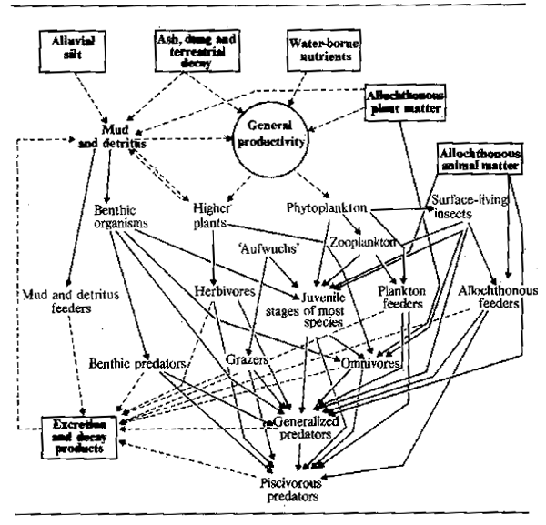
Figure 6.2 Diagram of trophic relationships in a river-floodplain community. Broken line = influence; Solid line = feeding interaction
| Main river channel bottom | Floodplain pools and lagoons | ||||||||
|---|---|---|---|---|---|---|---|---|---|
| Trophic category | Surface | Mud | Sand | Bank vegetation | Surface | Bottom | Vegetated (swampy) area | ||
| Mud and detritus feeders | Heterotis niloticus | Synodontis schall | Clarias ebriensis | Heterobranchus longifilis | Clarias ebriensis | ||||
| Citharinus latus | Labeo senegalensis | Heterobranchus longifilis | Heterotis niloticus | Neolebias unifasciatus | |||||
| Labeo ogunensis | Auchenoglanis occidentalis | ||||||||
| Synodontis schall | Phractolaemus ansorgii | ||||||||
| Citharinus latus | |||||||||
| Synodontis schall | |||||||||
| Herbivores micro | Labeo senegalensis | Synodontis nigrita(Juv) | Oreochromis galileus | ||||||
| macro | Distichodus rostratus | Distichodus rostratus | |||||||
| Tilapia guineensis | Tilapia guineensis | ||||||||
| Zooplankton | Pellonula afzeliusi | ||||||||
| Allochthonous and neston feeders | Brycinus longipinnis | Brycinus macrolepidotus | Epiplatys bifasciatus | ||||||
| Epiplatys sexfasciatus | |||||||||
| Omnivores | Brycinus nurse | Marcusenius brucii | Clarias lazera | Synodontis nigrita | Clarias lazera | ||||
| Chrysichthys auratus | Protopterus annectens | ||||||||
| Chrysichthys walkeri | |||||||||
| Synodontis melanopterus | |||||||||
| Synodontis nigrita | |||||||||
| Micropredators | Synodontis sorex | Synodontis sorex | Chromidotilapia guntheri | Chromidotilapia guentheri | Ctenopoma kingslayae | ||||
| Physailia pellucida | Petrocephalus bane | Brienomyrus brachyistius | Thysia ansorgii Barbus | ||||||
| Hyperopisus occidentalis | Petrocephalus bovei | Hemichromis bimaculatus | callipterus Pollimyrus | ||||||
| Mormyrus rume | Cyphamyrus psittacus | adspersus | |||||||
| Brienomyrus niger | Eutropiellus buffei | ||||||||
| Pollimyrus petricolus | |||||||||
| Pollimyrus adspersus | |||||||||
| Generalized predators | Schilbe mystus | Chrysichthys nigrodigitatus | Protopterus annectens | Malapterurus electricus | Calamoichthys calabaricus | ||||
| Eutropius niloticus | Calaraoichthys calabaricus | ||||||||
| Piscivores | Hydrocynus forskahlii | Bagrus docmac | Hemichromis fasciatus | Hepsetus odoe | Parachanna africanus | Hemichromis fasciatus | |||
| Lates niloticus | Polypterus senegalus | Polypterus senegalus | |||||||
| Hydrocynus vittatus | Gymnarchus niloticus | Gymnarchus niloticus | |||||||
| Hepsetus odoe | Parachanna obscurus | ||||||||
| Parachanna obscurus | |||||||||
In temperate rivers and streams the onset of winter usually marks a drop in overall productivity of aquatic system and in the production of food organisms. Furthermore, the amount of food eaten by fishes is closely related to temperature thus a general cessation of feeding occurs in most temperate and arctic species during the winter months. In tropical waters the effects of temperature are clearly less pronounced but since Chevey and Le Poulain (1940) remarked on the fact that fish did not feed in the Mekong system during the dry season it has become generally accepted that feeding by fish in tropical rivers is likewise highly seasonal all over the world. In flood rivers the feeding cycle is clearly linked to two factors, firstly the food supply and secondly the population density. During the flood the rapid increase in food organisms, together with the wide dispersal of fish over an extensive biotope, favours intensive feeding. At low water, when the aquatic environment is contracted the fish are concentrated in a few permanent reserves of water and food sources are limited or exhausted, fasting therefore ensues. In the tropics this contrasts with the more or less continuous feeding of fish in lakes; although in some species inhabiting rivers closely allied to lakes such as the Lake Chad/Yaeres system the fish cease feeding at low water despite the adequate supply of food which would enable them to continue feeding at all times of year. In reaches of Indian rivers having little or no floodplain the seasonality of feeding may be reversed with more intense food intake during the dry season. Bhatnagar and Karamchandani (1970) attributed this to the food being washed away by the high current during the flood in the case of Labeo fimbriatus. Tor tor showed a similar pattern to L. fimbriatus although in this case Desai (1970) correlated the lessened feeding with breeding. It would seem that feeding stops just before and during breeding in flood and reservoir rivers alike. There are nevertheless seasonal differences in the availability of food which depend on the morphology of the river.
The intensive feeding by fish during the periods of abundance permits them to build up large stores of fat which are sufficient, not only to tide the animals through the following barren winter or dry season, but to elaborate gonadial tissue in preparation for breeding. Starvation during the winter or dry season causes fish to lose condition. Daget (1956) for example traced this for Tilapia zillii in the Niger. Fig.6.3 shows the variation in weight over the dry season using condition factor K (where K = weight in gms x 105 over total length in mm³) as an index of change. In the river relatively little change occurred over the dry season until the start of reproduction when there was a sudden reduction in weight corresponding to about 10.7 percent for the whole period. In a floodplain pool fish ended the flood in better condition but lost weight more evenly throughout the dry season: in October and November - fish were fat and full of food (K = 4.52); in December - feeding was reduced (K = 4.68); January - stomachs empty (K = 4.67); February - very little food (K = 4.39); March - even less food (K = 4.48); April - only mud (K = 4.34); May (K = 4.16); June (K = 4.2). The net loss in weight over five months was 11 percent. In a second, somewhat richer, pool the loss in weight was less rapid (dashed line). Daget (1952) had previously noted similar seasonal changes in weight with Brycinus. In the Amazon, Junk (in press) observed seasonal changes in the fat content of 40 species. The majority of these showed a pronounced seasonality in chemical composition with peaks in fat content during the falling flood and minimum fat content during the breeding season at the end of low water.
The pattern of abundant feeding during the flood and fasting during low water is, perhaps, not as simple as it appears. Observations by Willoughby and Tweddle (1978) indicated that peak feeding takes place at different times in different species (Fig. 6.4). The food consumption of Clarias gariepinus in the Shire system, for instance, reached its maximum just before the flood peak, whereas Oreochromis mossambicus fed more intensively as the floodplains were draining. A third species, Clarias ngamensis, fed at a fairly constant rate for most of the year. In all three species food intake was minimal at low water. There are also indications that certain categories of feeders continue to feed throughout the dry season. Microvores such as Heterotis niloticus may feed throughout the year, although only at maintenance level during the dry season (Daget, 1957a). Surface feeders also have a continuing food source and Brycinus macrolepidotus continues to feed long after other species of Alestes and Brycinus in the Niger. The change in predator-forage fish ratio throughout the dry season, and the gradual disappearance of smaller fishes from floodplain pools, as noted by Lowe-McConnell (1964) would suggest that predators may continue feeding well into the dry season. Goulding (1980) also found that, whereas the majority of frugivorous Amazonian fish greatly reduced their feeding during the low water seasons, the predatory characins were less inclined to do so in that roughly equal proportions of such fish contained food in the dry and wet seasons. However, the nature of the food changed from primarily plant foods (seeds and fruit) in the wet season to fish scales in the dry. Neverthless, predators appear to stop feeding in other systems and Mago-Leccia (1970), in noting that Piranhas turn to mud as a feeding substrate in the dry season, also remarked that small fish are not eaten by predators at low water. Such continued feeding does appear to be somewhat exceptional and most observers confirm the dry season fast.
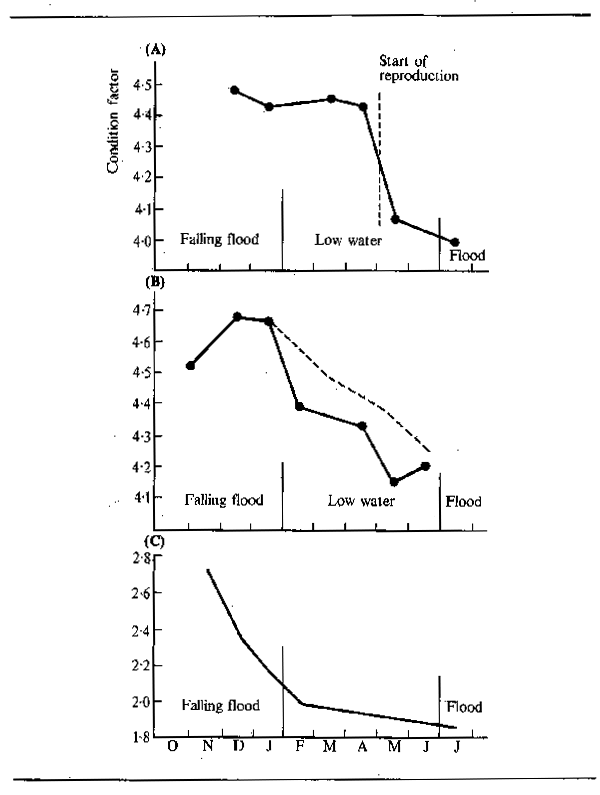
Figure 6.3 Changes in condition factor between October and July for adult Tilapia zillii in: (A) the Niger River, and (B) two floodplain pools (after Daget, 1956). Also shown are (C) changes in condition factor of Brycinus leuciscus (after Daget, 1957a)
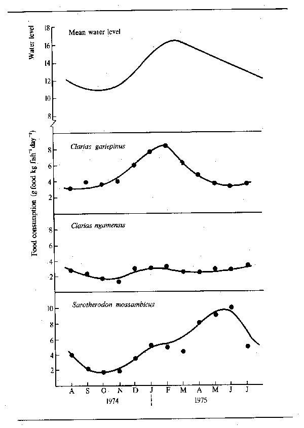
Figure 6.4 Seasonal variations in daily food intake by three species of fish from the Shire River. (After Willoughby and Tweddle, 1978)
Fish from most river systems show well-defined rings or annuli on their scales, bones or otoliths, a fact which has been noted from tropical and subtropical systems as well as from temperate ones. The rings of temperate salmonid and coarse fish species have been widely described. Chevey and Le Poulain (1940) noted rings on the scales of cyprinid species in the Mekong, and rings have been described from other cyprinids such as Labeo spp. in both the Gambia (Johnels, 1954) and Indian rivers (Khan and Jhingran, 1975), or Catla catla from the Ganges (Natarajan and Jhingran, 1963). Numerous characin species have been studied, Prochilodus scrofa (Godoy, 1975), P. platensis is (Cabrera and Candia, 1964; Vidal, 1967) in South America, and Brycinus leuciscus (Daget, 1952) and Alestes baremoze (Durand and Loubens, 1969) in Africa. Cichlids from both Africa (Oreochromis spp., Dudley, 1972) and Latin American rivers (Cichlasoma bimaculatum, Lowe-McConnell, 1964) have been recorded with annuli on their scales. Johnels (1954) also mentions rings on the scales of Notopterus sp. and mormyrids. Other hard parts of the fish also show qrowth rings. Opercular bones were used by Cordiviola (1971) for ageing Prochilodus platensis. The scaleless siluroids (Candia et al., 1973) have shown clear rings in the otoliths and pectoral spines of Parapimelodus valenciennesi and Fenerich et al., (1975) have demonstrated their existence in the otoliths of Pimelodus maculatus. Pectoral spines and vertebrae were used to age Clarias spp. from the Kafue flats by the University of Idaho et al. (1971). Other growth studies, such as those by Bayley (1983) for 12 species of the Amazon system, have been based on length frequency analyses without recourse to structures.
The marks or rings have been correlated with the partial or complete cessation of growth during one or more periods of the year. In the temperate zone these are clearly associated with the winter cessation of growth. However, in the tropics more rings have often been recorded than would be expected if ring formation depended solely on a regular seasonal event. Care therefore has to be taken in interpreting rings in scales or other hard structures as indicators of age or time series. Nevertheless at low water feeding either stops completely or is seriously reduced in most species. The fish live on their fat reserves, sometimes losing condition to the point where resorption occurs at the margin of the scales. Durand and Loubens (1969) made a useful distinction between growth in weight and growth in length. The latter is a good indicator of long-term change, but as it depends mainly on skeletal structures it is not so liable to modification during the growth arrest. Growth in weight is as much through the addition of soft tissues including fat. These fat stores are liable to be rapidly modified under adverse conditions, as has been shown for Tilapia zillii and Brycinus leuciscus (Fig. 6.3), and as Durand and Loubens (1970) showed for Alestes baremoze, where the condition factor (K) fell from 1.30 in April to 1.00 in September. Of course care has to be taken in the interpretation of changes in weight and condition factor, as the development of gonadial tissue and discharge of eggs or milt is also reflected in these parameters. However, changes in K are more often slow over the whole dry period, than abrupt at the time of breeding, as would be the case if the discharge of reproductive products were the sole cause.
Three main reasons have been advanced for the arrest of growth during several months of the year.
(i) temperature
(ii) effects associated with drawdown; and
(iii) reproduction
In the temperate zone, temperature is clearly the dominant feature and ring formation is correlated with winter but the growth rate arrest coincides with a drop in temperature. In several tropical river systems too, for instance, in the Lake Chad basin, winter temperatures drop at least 8°C below the summer maxima (Durand and Loubens, 1969) and coincide with the minimum growth rate. Similarly in the Senegal, Reizer (1974) considered the slower growth from December to February to be correlated with lower temperatures, and in both the lower La Plata system and on the Kafue flats, the minimum rate of growth occurs at the same time as similar drops in temperatures. In most of these rivers, however, low water coincides with the winter and it is difficult to distinguish the effects of the two factors. In the southern Okavango swamps the floods arrive during the colder part of the year (Fox, 1976) which leads to very low growth rates of the fish living there. It is not yet clear when the growth arrest occurs in these waters, although current work may shed some light on this.
In equatorial rivers growth checks occur regularly where there are only mimimal changes in temperature. In such circumstances Lowe-McConnell (1964) has suggested that crowding and lessened availability of food, brought about by drawdown conditions, are responsible. That this too cannot be the whole answer is shown by the Lake Chad fishes which stop growing in the lake even though there is abundant food. In the Niger river (Daget, 1957) reported that growth arrests can be distinguished on the scales of carnivores, herbivores, limnivores, insectivores and plankton-eating species, despite the fact that the predators and limnivores at least have sufficient food. Furthermore, some fish such as the young of Oreochromis and Tilapia in the Kafue, resume feeding before the onset of the floods, at a time when conditions are at their most cramped (Dudley, 1974).
The effects of population density on growth rate are somewhat problematic. In the Danube, Chitravadivelu (1974) was unable to detect changes in the growth rate of Alburnus alburnus and Rutilus rutilus, despite great differences in biomass and population density from one year to another. However, Frank (1959) did record increases in growth in Rutilus rutilus and Abramis brama when the population decreased from 69 124 i/ha to 19 394 i/ha in an Elbe oxbow. This he traced to the greater availability of planktonic food following the decline in competition for this food source. Clear relationships between population density and the growth rate and the total production of bullhead (Cottus gobio) have also been demonstrated by Edwards and Brooker (1982), (Fig. 6.5) from tributaries of the river Wye. Similar experiments with brown trout show a pronounced drop in individual growth rate as the number of fish present per unit area increases (Backiel and Le Cren, 1978). Such conflicting results indicate a need for further investigation into the question of the relationship of food supply to population density, as this influences the amount of fish available to the fishery.
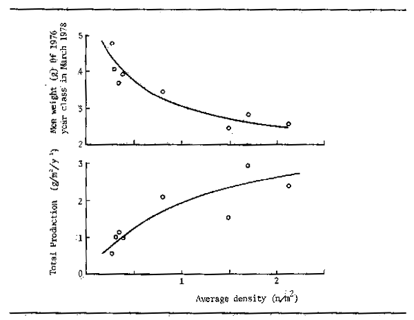
Figure 6.5 Relationships between density and (A) growth, and (B) production in bullhead (Cottus gobio) in tributaries of the Upper Wye. (From Edwards and Brooker, 1982)
The elaboration of gonadial products during the fasting period probably accelerates the depletion of fat reserves and exaggerates the low physical condition which is reflected as an annulus. It is, however, doubtful whether this is the prime reason for growth checks, as maturation is frequently preceded by a long period of negligible feeding in many species. Furthermore, rings are laid down by immature fish as well as adults. That there may be deep physiological rhythms which dictate the seasonal cessation of growth is suggested by an isolated experiment quoted by Johnels (1954). Here some Barbus gambiensis, which had been transported to Sweden and were being maintained in the even conditions of an aquarium, still stopped growing and laid down scale rings at precisely those times when their congeners did so in the Gambia river.
Annuli on scales and other hard parts have been used to calculate growth in many species. Supplementary information and independent estimates of growth have also been made from the analysis of length frequency distributions for the progression of individual age groups and also from the growth of tagged fish. Comparisons between the various methods of age determination show that they give good agreement at least in sane species (Rao and Rao, 1972; Gupta and Jhingran, 1973). Several workers have used the Von Bertalanffy model of growth:

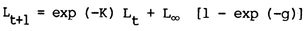
in which length at time t + 1(Lt+1) is a function of length at time t (Lt) according to the Ford-Waiford equation:
where K is the coefficient of growth and Lo the theoretical asymptotic length achievable by the species if it grows for an infinite period of time.
Most species seem to conform well to this model in respect of growth in length, or when subject to an appropriate conversion factor, in respect of growth in weight, as is shown by examples in Table 6.4.
| Species | Sex | Growth equation | Author |
|---|---|---|---|
| Alestes baremoze | ♂ | Lt=237.8[1-e-0.8163(t-0.57)] | Durand and Loubens, 1969 |
| ♀ | Lt=267[1-e)-0.7172(t-0.52)] | Durand and Loubens, 1969 | |
| Catla catla | ♂ + ♀ | Lt=1275[1-e)-0.28(t-0.11)] | Natarajan and Jhingran,1975 |
| Labeo rohita | ♂ + ♀ | Lt=1015[1-e)-0.276(t-0.333)] | Khan and Jhingran, 1975 |
| Labeo calhasu (Ganga river) | ♂ + ♀ | Lt=1028[1-e)-0.15(t-0.19)] | Gupta and Jhingran, 1973 |
| (Godavari river) | ♂ + ♀ | Lt=944[1-e)-0.14(t+0.86)] | Rao and Rao, 1972 |
| Parapimelodus valenciennesi | ♂ + ♀ | Lt=333[1-e)-0.14(t-2.4)] | Candia et al., 1973 |
| Pimelodus maculatus | ♂ | Lt=45.4[1-e)-0.2104(t-0.61)] | Fenerich et al., 1975 |
| ♀ | Lt=56.5[1-e)-0.1938(t+0.36)] | Fenerich et al., 1975 | |
| Prochilodus reticulatus | ♂ + ♀ | Lt=41.0[1-e-0.20(t-0.35)] | Espinosa and Gimenez, 1974 |
From the table it may be seen that male and female fish of the same species freQuently have different rates of frowth and also maximum sizes as indicated by L∞. Growth curves of some representative species from an African river (Niger) and the Latin American La Plata system shows part of the range of interspecific variation (Fig. 6.6). Most species grow very rapidly in their first season, a feature which Dowe-McConnell (1967) regarded as adaptive. Predation is intense in floodplain rivers, so rapid growth to get to a size too large to be swallowed before the shelter of the floating vegetation on the floodplain disappears, is a great advantage. Fish probably also need to attain an adequate size to migrate by the time the floods recede. There seems to be little difference in the size attained by year 1 in fish having a wide range of maximum sizes as shown by Merona (1983) in his examination of over 100 African species.
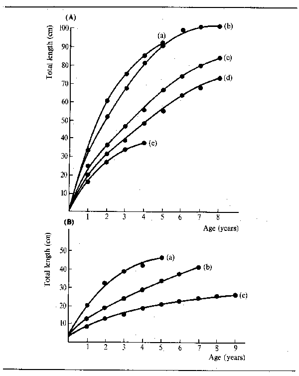
Figure 6.6 Growth in length of representative fishes from rivers: (A) Niger: (i) Heterotis niloticus; (ii) Lates niloticus; (iii) Mormyrops deliciosus; (iv) Citharinus citharus; (v) Eutropius niloticus (B) La Plata: (i) Prochilodus platensis (after Cordiviola de Yuan, 1971); (ii) Pimelodus maculatus (after Fenerich et al., 1975); (iii) Parapimelodus valenciennesi (after Cabrera et al., 1973)
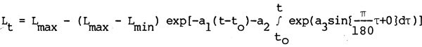
Whereas the Von Bertalanffy growth curve adequately describes year to year progression in length, growth within any one year does not conform to the model. The long period in which growth either ceases completely or is considerably restricted, means that most of the year's increase in length occurs during a comparatively short period. Dudley (1972), for instance, recorded that 75 percent of the expected first years growth of Oreochromis andersoni and O. macrochir took place within six weeks of peak floods in the Kafue river. Growth in weight is even more subject to seasonal variation, often with temporary losses occurring during the dry season.
Because the within-the-year growth pattern has important implications for the estimation of biological production, Daget and Ecoutin (1976) have produced a modified growth model applicable to species with prolonged annual growth arrests. This requires the introduction of two new parameters into the growth equation. These are q, which represents the duration of the annual growth arrest in months, and t, which is the duration of the first period of growth also in months. The parameter t is necessary where reproduction does not coincide with the end of the parent's period of arrested growth. When the growing period is 12 - q months, the normal Von Bertalanffy curve is expressed as:
Lt = L∞ {1 exp [-g' (t-to)]}
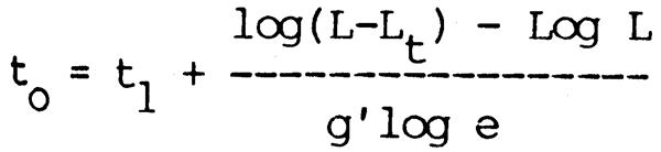
where t and tO are expressed in months and g' = g/12-q; tO is obtained from the equation
The arc of the growth curve thus obtained is thereby compressed into 12-q months and is followed by a horizontal line q months long. Daget and Ecoutin applied this model to Polypterus senegalus from the Middle Niger obtaining the mean growth curve shown in Fig. 6.7. A similar modification of Von Bertalanffy's model was proposed by Cloern and Nichols (1978) to take into account seasonal variations in growth rate in temperate waters. This model:
where L is length at time (t), L max is maximum body size, L min is body size at time of recruitment obtains growth predictions with a much smoother transition from growth to arrest phases.
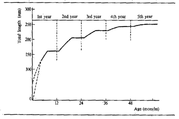
Figure 6.7 Mean linear growth of Polypterus senegalus for the first five years of life assuming an annual growth arrest of six months and a first year's growth period of seven months (T0 = -3). (After Daget and Ecoutin, 1976)
These models describe situations where growth stops completely during the dry season and have the advantage of being based on current growth models, but are somewhat inflexible when applied to situations where growth varies from year to year depending on favourable or unfavourable conditions. Such conditions require a growth trajectory that is less pre-determined, and Welcomme and Hagborg (1977) had to adopt a different model for growth within the year to allow for this. Their formula: has the characteristics of fast initial increase in length followed by a period of slower growth (but not a complete halt). Values of Lt for successive years can conform to the Von Bertalanffy relationship, although the form of the curve within one year calculated for successive weeks does not. The advantage of this relationship in modelling the growth of fish living on floodplains, is that the terminal value of the years growth can change according to the intensity of flooding by the operation of an appropriate coefficient on G.
Lt+t1 = Lt + G exp(t1)
In his studies on fish production in the Kafue river, Kapetsky (1974 and 1974a) was presented with a similar problem of modelling within year growth patterns. From his own observations as well as those of Dudley (1972) it was obvious that growth in weight of Sarotherodon and Oreochromis spp. on the Kafue flats does not stop completely in the dry season, although it is considerably slowed. Kapetsky, therefore, proposed to rotate the relationship Wt = WO exp(Gt) on its diagonal and then reverse it. This gives an equation of the form:
Wt = WO + W1 [1 - exp(-gt)]
where W1 = W0 exp G(12). Here W1 = the weight at the end of a year's growth, whereas individual segments of t and the growth coefficient g are in months.
There appear to be few studies on interannual variation in growth rate of fish from the rhithron and from low order streams of the temperate zone. It may be assumed that, given the relatively stable conditions of such environments between years, similar rates of growth are obtained. However, there are indications that density dependant factors may influence the rate of growth in some species, although the origin of the fluctuations are not clear.
From the studies of growth of fish species inhabiting the potamon it has become obvious that there are considerable year-to-year variations in growth within the same species. The most detailed examination of the possible causes of such variations has been carried out for some cichlid species in the Kafue river. Here, Dudley (1972 and 1974) and Kapetsky (1974) found significant correlations between some physical variables and the main growth increment. The intensity and duration of flooding particularly could have accounted for much of the year-to-year variation in the growth of year class I and II, Tilapia rendalli, Oreochromis andersoni and O. macrochir. Low temperature in the dry season also appeared to influence some year classes and gave good partial correlations when entered into the equation after some measure of flood intensity. Typical relationships are shown in Table 6.5 where TI is an index of temperature, FI is an index of flooding drawn from the area under the flood curve (Dudley 1972), and HI 2 and HI 3 are indices summarizing the degree of drawdown in the dry season (Kapetsky, 1974).
Kapetsky's regression equations were successfully used to predict growth increments for certain year classes, but the consistency of the results is not uniform, possibly due to the short time series upon which the calculations were based. They are sufficient, however, to indicate the importance of external physical factors in determining the growth of fish in such systems. This work on the Kafue is not isolated. As early as 1934 Wimpenny (quoted in Holden, 1963) found that the yield of fish from the Nile delta, Lake Manzala, was correlated with flood level, high floods being followed by better than average yields which were due in part to higher growth rates of first year fish. Similarly, conditions for feeding, and hence growth, of non-anadromous fishes in the Amur river are considerably improved in years when there is plenty of water (Krykhtin, 1972, quoted by Krykhtin, 1975). The exceptionally poor flood years during the 1968–74 Sahelian drought provided an opportunity to assess the effects of this on the growth of fish species in the Senegal, Niger and Logone rivers. In the Senegal, Reizer (1974), discerned great differences in growth of Citharinus citharus between 1968, a year of particularly poor flood, and other years (Fig. 6.8). The first year class was missing totally for that year. The second year growth increment for the 1967 year class in the 1968 flood was 3.91 cm, whereas the 1966 year class grew 7.99 cm during the 1967 flood. The third year's growth showed similar differences; an increment of 2.32 cm for the 1966 year class (1968 flood) and 8.37 cm for the 1967 year class (1969 flood). Differences in growth were also noted from the Niger where the floods of 1971 and 1972 were particularly bad. Here Dansoko (1975) and Dansoko et al. (1976) studied two species of Hydrocynus, H. brevis and H. forskahlii, and found that growth, particularly of the young of the year in both species, was poor during these two years. Hydrocynus forskahlii, which only inhabits the river, showed this effect less that H. brevis which depends much on the floodplain for feeding, but nonetheless the differences were still marked. It is also of interest that year classes with poor first year growth appear to continue to grow badly despite better conditions in later years. Likewise year classes with good initial growth do not suffer so badly in poor years. In the Logone Benech and Quensiere (1984) were also able to demonstrate improved growth, as represented by the mean weight of fish leaving the Yaeres floodplain through the El Beid, as a correlate of the Logone flood in several species including Hyperopisus bebe, Brachysynodontis batensoda, Marcusenius cyprinoides, Oreochromis aureus and O. niloticus.
| Species | Year of growth | Sex | Model | r |
|---|---|---|---|---|
| Oreochromis andersoni | 1 | M | Growth (cm) = 0.02FI+12.87 a | 0.92 |
| 1 | M | TL (mm) = 146.51–0.11(HI2) b | 0.94 | |
| 1 | F | Growth (cm) = 0.014FI+13.4 a | 0.78 | |
| 2 | M | TL (mm) = -29.47+1.98 (TI) b | 0.90 | |
| 2 | F | TL (mm) = 38.24–0.30(HI3)+0.83(TI) b | 0.93 | |
| Oreochromis macrochir | 1 | M | Growth (cm) = 0.2FI+11.02 a | 0.9 |
| 1 | M | TL (mm) = 130.39–0.13(HI2) b | 0.92 | |
| 1 | F | TL (mm) = 130.13–0.32(HI2) b | 0.85 | |
| 2 | M | TL (mm) = 74.72.0.10(HI3) b | 0.58 | |
| 2 | F | TL (mm) = 14.69–0.18(HI3) b | 0.95 | |
| Tilapia rendalli | 1 | M | Growth (cm) = 0.029FI+12.8 a | 0.80 |
a Dudley, 1972
b Kapetsky, 1974
Figure 6.8 Growth of Citharinus citharus in the Senegal river: 1966, 1967, 1969 year classes. Numbers in parentheses = total length at growth arrest in centimetres. (After Reizer, 1974)
Fish inhabiting rivers show a diversity of reproductive habit which adapts them to the varying conditions encountered along the length of the river and to the particular difficulties inherent in breeding in systems with rapidly fluctuating water levels and often extreme conditions of flow or oxygen deficiency. It seems that physical and behavioural specializations for reproduction are more varied than those for feeding in these ecosystems. The range of adaptations is indicated by the fact that nearly all of Balon's reproductive guilds (Balon 1975 and 1981) are represented in the various rivers of the world. These guilds which form a useful ecological classification of breeding behaviour, localities and substrates are listed in Table 6.6 together with some representative taxa. Several broad reproductive strategies have evolved within these guilds which are summarized in Table 6.7.
| Ethological section - A. Nonguarders |
|---|
A.1 Open substratum spawners
(Selected key features of early ontogeny)
Pelagic spawners (pelagophils)
Numerous buoyant eggs, none or poorly developed embryonic respiratory organs, little pigment, no photophobia. Ctenopoma muriei, Lates niloticus.
Rock and gravel spawners with pelagic larvae (lithopelagophils)
Adhesive chorion at first, some eggs soon buoyant, after hatching free embryos pelagic by positive buoyancy or active movement, no photophobia, limited embryonic respiratory structures. Prochilodus spp.
Rock and gravel spawners with benthic larvae (lithophils)
Early hatched embryo photophobic, hide under stones, moderately developed embryonic respiratory structures, pigment appears late. Many cyprinid and characin spp., Barbus and Labeo.
Nonobligatory plant spawners (phytolithophils)
Adhesive eggs on submerged items, late hatching, cement glands in free embryos, photophobic, moderately developed respiratory structures. Many cyprinids and Rutilus rutilus.
Obligatory plant spawners (phytophils)
Adhesive egg envelope sticks to submerged live or dead plants, late hatching, cement glands, not photophobic, extremely well developed embryonic respiratory structures. Many cyprinid, characin and siluroid spp., Puntius gonionotus.
Sand spawners (psammophils)
Adhesive eggs in running water on sand or fine roots over sand, free embryos without cement glands, phototropic, feebly developed respiratory structures, large pectorals, large neuromast rods (cupulae). Many migration cyprinid and characin spp.
Terrestrial spawners (aerophils)
Small adhesive eggs scattered out of water in damp sod, not photophobic, moderately developed respiratory structures. Brycon petrosus.
A.2 Brood hiders
Beach spawners (aeropsammophils)
Spawning above the waterline of high tides, zygotes in damp sand hatch upon vibration of waves, pelagic afterwards. Not represented.
Annual fishes (xerophils)
In cleavage phase blastomeres disperse and rest in first facultative diapause, two more resting intervals obligate - eggs and embryos capable of survival for many months in dry mud. Nothobranchius.
Rock and gravel spawners (lithophils)
Zygotes buried in gravel despressions called redds or in rock interstices, large and dense yolk, extensive respiratory plexuses for exogenous and carotenoids for endogenous respiration, early hatched free embryos photophobic, large emerging alevins. Many salmonid species.
Cave spawners (speleophils)
A few large adhesive eggs, must hide in crevices, extensive embryonic respiratory structures, large emerging larvae.
Spawners in live invertebrates (ostracophils)
Zygotes deposited via female's ovipositor in body cavities of mussels, crabs, ascidians or sponges, large dense yolk, lobes or spines and photophobia to prevent expulsion of free embryos, large embryonic respiratory plexuses and carotenoids, probable biochemical mechanism for immunosuppression. Rhodeus sericeus.
Ethological section - B. Guarders
B.1 Substrate choosers
Pelagic spawners (pelagophils)
Nonadhesive, positively buoyant eggs, guarded at the surface of hypoxic waters, extensive embryonic respiratory structures. Some Ophicephalus and Anabas spp.
Above water spawners (aerophils)
Adhesive eggs, embryos with cement glands, male in water splashes the clutch periodically. Copeina arnoldi.
Rock spawners (lithophils)
Strongly adhesive eggs, oval or cylindrical, attached at one pole by fibres in clusters, most have pelagic free embryos and larvae. Loricaria parva, L. macrops and some small cichlids.
Plant spawners (phytophils)
Adhesive eggs attach to variety of. aquatic plants, free embryos without coment glands swim instantly after prolonged embryonic period. Polypterus spp.
B.2 Nest spawners
Froth nesters (aphrophils)
Eggs deposited in a cluster of mucous bubbles, embryos with cement glands and well developed respiratory structures. Hepsetus odoe, Hoplosternum, some anabantids.
Miscellaneous substrate and material nesters (polyphils)
Adhesive eggs attached singly or in clusters on any available substratum, dense yolk with high carotenoid contents, embryonic respiratory structures well developed feeding of young on parental mucus common. Notopterus chitala, Hoplias malabaricus.
Rock and gravel nesters (lithophils)
Eggs in spherical or elliptical envelopes always adhesive, free embryos photophobic or with cement glands swing tail-up in respiratory motions, moderate to well developed embryonic respiratory structures, many young feed first on the mucus of parents. Aequidens and other cichlids, some characins, e.g., Leporinus.
Gluemaking nesters(ariadnophils)
Male guards intensively eggs deposited in next bind together by a viscid thread spinned from a kidney secretion, eggs and embryos ventilated by male in spite of well developed respiratory structures. Gasterosteus aculeatus
Plant material nesters (phytophils)
Adhesive eggs attached to plants, free embryos hang on plants by cement glands, respiratory structure well developed in embryos assisted by fanning parents. Clarias batrachus.
Sand nesters (psammophils)
Thick adhesive chorion with sand grains gradually washed off or bouncing buoyant eggs, free embryo leans on large pectorals, embryonic respiratory structures feebly developed. Tilapia spp.
Hole nesters (speleophils)
At least two modes prevail in this guild: cavity roof top nesters have moderately developed embryonic respiratory structures, while bottom burrow nesters have such structures developed strongly. Several cichlids.
Anemone nesters (actiniariophils)
Adhesive eggs in cluster guarded at the base of sea anemone, parent coats the eggs with mucus against nematocysts, free embryo phototropic, planktonic, early juveniles select host anemone. Not represented.
Ethological section - C. Bearers
C.1 External bearers
Transfer brooders
Eggs carried for some time before deposition; in cupped pelvic fins, in a cluster hanging from genital pore, inside the body cavity (earlier ovi ovoviviparous), after deposition most similar to nonguarding phytophils. Callichthys, Corydoras.
Auxiliary brooders
Adhesive eggs carried in clusters or balls on the spongy skin of ventrum, back, under pectoral fins or on a hook in the superoccipital region, or encircled within coils of female's body, embryonic respiratory circulation and pigments well developed. Loricaria spp.
Mouth brooders
Eggs incubated in buccal cavity after internal, external synchronous or asynchronous, or bucca fertilization assisted by egg dummies, large spherical or oval eggs with dense yolk are rotated (churning) in the cavity or densely packed when well developed embryonic respiratory structures had to be assisted by endogenous oxydative metabolism of carotenoids, large young released. Many cichlids, Osteoglossum.
Gill-chamber brooders
Eggs of North American cavefishes are incubated in gill cavities.
Pouch brooders
Eggs incubated in an external marsupium: an enlarged and everted lower lip, fin pouch, or membraneous or boy plate covered ventral pouch, well developed embryonic respiratory structures and pigments, low number of zygotes. Loricaria vetula and L. anus.
C.2 Internal bearers
Facultative internal bearers
Eggs are sometimes fertilized internally by accident via close apposition of gonopores in normally oviparous fishes, and may be retained within the female's reproductive system to complete some of the early stages of embryonic development, rarely beyond the cleavage phase; weight decreases during embryonic development. Rivulus marmoratus, Oryzias latipes, Pantodon buchholzi.
Obligate lecithotrophic livebearers
Eggs fertilized internally, incubate in the reproductive system of female until the end of embryonic phase or beyond, no maternal-embryonic nutrient transfer; as in oviparous fishes yolk is the sole source of nourishment and most of the respiratory needs; some specialization for intrauterine respiration, excretion and osmoregulation; decrease in weight during embryonic development. Poeciliopsis monacha, Poecilia reticulata, Xenopoecilus poptae.
Matrotrophous oophages and adelphophages
Of many eggs relased from an ovary only one or at most a few embryos develop into alevins and juveniles, feeding on other less developed yolked ova present and/or periodically ovulated (oophagy), and in more specialized forms, preying on less developed sibling embryos (adelphophagy); specialization for intrauterine respiration, secretion and osmoregulation similar to the previus guild; large gain in weight during intrauterine development.
Viviparous trophoderms
Internally fertilized eggs develop into embryos, alevins or juveniles whose partial or entire nutrition and gaseous exchange is supplied by the mother via secretory histotrophes ingested or absorbed by the fetus via epithelial absorbative structures (placental analogues) or a yolksac placenta; small to moderate gain in weight during embryonic development. Poeciliopsis turneri, Heterandria formosa, Anableps dowi.
| Type of fecundity | Seasonality | Examples | Movement and parental care |
|---|---|---|---|
| Big bang | Once in a life-time | Anguilla | Very long catadromous migrations, no parental care |
| Total spawners (very high fecundity) | Highly seasonal concentrated on annual or bi-annual floods | Characins: e.g. Prochilodus, Salminus, Alestes | Long distance migrants, open substratum spawners |
| Cyprinids: e.g. Labeo, Barbus, Cirrhinus | |||
| Siluroids: e.g. Schilbe | |||
| Heteropneustes, Catla catla, Labeo rohita | Local lateral migrants open substratum spawners | ||
| Mormyrids | |||
| Partial spawners | Throughout flood season(s) | Some cyprinids, characins and siluroids: e.g. Clarias, Micro- alestes acutidens | Mainly lateral migrants: open substratum spawners |
| Grades into | Protopterus, Arapaima, Serrasalmus, Hoplias, Heterotis | Bottom nest constructors and guarders | |
| Ophicephalus, Gymnarchus | Floating nest builders | ||
| Hepsetus Hoplosternum Anabantids, | Bubble nest builders | ||
| Small brood spawners (low fecundity) | High water but may start during low water or may continue throughout the year | Tilapia, Hypostomus | Nest constructors with various behavioural patterns |
| Aspredo, Loricaria sp. | Egg carriers | ||
| Osteoglossum, Sarotherodon spp. | Mouth brooders | ||
| Potamotrygon, Poeciliids | Live bearers | ||
| End of rains | Some cyprinodonts | Annual species with resting eggs |
Fish spawning within rhithronic reaches of the main channel usually have to contend with high flow and turbulence. Consequently they tend either to have adhesive eggs which stick to rocks and plants (lithophils or phytophils) or to place the eggs in crevices of the rocky substrates of the riffles (lithophils). Some salmonids for instance cut “redds” into fine gravel which are designed both to protect and aerate the eggs. Other species spawning in small streams may lay their eggs in very shallow water or in damp terrestrial environments (aerophils). For example, the group spawning Brycon petrosus is described by Kramer (1978) as lodging its eggs in the splash zone at the margins of Panamanian streams. Several other species including Fundulus similis, F. heteroclitus and Hypomesus pretiosus also have similar behaviour. Other fish from the Amazon, Madeira, Orinoco, Danube and Amur as well as presumably many other rivers which spawn in the main channel have semibuoyant eggs (lithopelagophils) which drift downstream with the current until finding suitable feeding grounds usually on floodplains or backwaters.
Many species migrate considerable distances upstream in order to spawn in the rhithronic lower order streams where presumably the good aeration, rich food supply of the riffles and relative freedom from predation all favour the development of the fry. To compensate for the high risks inherent in these environments however nearly all species spawning in such regions produce large numbers of eggs and are total spawners. That upstream migrants do not all seek the same type of headwater is shown by the observations made by INDERENA (1973) on the Magdalena river. Here Brycon moorei moved into small short side arms off the main channel, whereas Prochilodus reticulatus stayed within the main channel, Salminus affinis swam up side streams to areas of high flow and Brycon henni ascended to the highest accessible reaches of the main river.
In Europe breeding success of some species appears mainly dependent on the presence of suitable substrates. Even under considerably modified hydrological regimes species such as Rutilus rutilus or Abramis brama have shown themselves capable of changing from the type of migratory behaviour they show in the Volga or Lower Danube to their more static behaviour in Western European modified streams provided the required substrates are available. Other species, such as Chandrostoma nasus, Barbus barbus or Leuciscus idus have shown themselves much less able to so adapt.
Migratory species may alter their reproductive strategy to adapt to different climatic conditions. For instance Alosa sapidissima, an anadromous species which enters rivers on the East coast of the United States to spawn, breeds more frequently, but releases few eggs per breeding in the cooler northern rivers than in the warmer southern rivers (Legget and Carscadden, 1978). This means that in northern rivers, more of the available energy is allotted to migration in order to place eggs and fry in the most favourable conditions. Legget and Carscadden add that available literature suggests that many other species are equally capable of fine tuning their reproductive strategies to accord with local environmental circumstances. Such behaviour would mean that populations specific to certain rivers would develop and that homing capabilities would be needed to ensure that the behavioural patterns would match the climatic conditions of the spawning environment.
The most diverse breeding strategies are found in those fish spawning on the floodplains, and many species migrate considerable distances up or downstream to breed so as to place their fry in these productive habitats. Utilization of the floodplain for spawning is in fact recorded from most tropical river systems and is also common in such temperate rivers as still have plains. Thus the various authors writing on larval fish distribution in the Mississippi-Missouri system (e.g. Kallemyn and Novotny, 1977) state that the floodable marsh areas of the backwaters are vital for the spawning of many species. Similar observations have also been made in the Danube (e.g., Holcik and Bastl, 1976) and the Volga (Koblitskaya, 1985).
Migratory blackfishes show a wide range of behaviour. Most are open stratum phytolithophils or phytophils which attach or scatter their eggs among vegetation or over open bottoms of the floodplain. Often the localities chosen for egg deposition are in the channels conducting water on to the plain as in the Alestes species of the Logone river which lay their eggs in the channels feeding the Yaeres floodplain while the adults themselves never penetrate the plain. Alternatively species migrating on to the floodplains of the Ayuthaya province of Thailand (Chao Phrya river system) illustrate the selection of substrates for spawning (Tongsanga and Kessunchai, 1966). Crossocheilus reba spawns in the inundated rice fields as does Wallago attu. Another catfish, Pangasius sutchi scatters its eggs among submerged weeds and bushes in the shallow inundated margins of the Klongs or canals. The spring eel Macrognathus aculeatus spawns both in flooded rice fields and in the channels on clear bottoms or among weeds. Some species, such as Puntius goniotus drop their eggs in the middle of channels and presumably rely on currents to wash them into suitable nursery sites.
Closely related species and genera also show contrasting behaviour. For example, Hydrocynus brevis breed on the floodplain of the Niger during the floods whereas the morphologically similar H. forskahlii breeds in the main river channel during low water. Jackson and Coetzee (1982) have remarked on the habits of S. African Labeo umbratus which move on to flooded grasslands to lay their sticky eggs among the temporarily submerged vegetation as contrasted to the local Barbus johnstoni and B. trapilepidotus which both spawn in gravel areas of swift flowing rivers. Their conclusion that these behaviour patterns can be enlarged to make a fundamental distinction between the two genera does not, however, stand up to closer inspection as some Labeo species, e.g. Labeo parvus of the Niger River which inhabit rapids breed in the riffle zones of the main channel and some small Barbus equally breed in the flooded grass of the floodplain.
Most blackfish species which at the most are only local migrants have some form of parental care and in some genera a variety of behavioural patterns are found. This is typified by the genus Loricaria, where L. parva and L. macrops sit on eggs which are attached to cleared areas of rock. The eggs are cleaned and fanned by the parents from time to time. Female L. piracicalae develop a special spongy skin on their ventral surface. The fish roll on the fertilized eggs which adhere to this region. L. vetula and L. anus have a pouch formed by the enlargement of the lower lip of the males in to which the eggs are lodged, and in Loricaria sp. (near microdon: Lowe-McConnell, 1964) the lower lip is extended into a special elongation from which the young are suspended. Other loricariids such as the Panamanian L. uracantha use hollows and cavities in pieces of wood as nesting sites (Moodie and Power, 1982).
Nest building is very common among floodplain species. Arapaima gigas scoops out hollows in the bottom of the flooded savanna and both parents .guard the eggs that are deposited (Sanchez, 1961). Various species of cichlid make nests. Some of these are simply cleared areas of rock, others holes under rocks or vegetation, and in yet others, excavated pits sometimes of complex design. Heterotis niloticus, construct nests in the middle of masses of vegetation at the shallow margins of the plain, whereas Gymnarchus niloticus make floating flask or raft shape masses of aquatic weeds in which they lay their eggs (Svensson, 1933). The different architecture of the nests of Protopterus has been described by Johnels and Svensson (1954) for P. annectens and Greenwood (1958) for P. aethiopicus. These range from simple sunken areas in a sandy substrate to complex domed structures of papyrus roots. The characin Hoplias malabaricus constructs a simple nest on the bottom with whatever material is readily available and some species of Serrasalmus are also reputed to guard egg masses laid on tree roots, and aquarium observations have shown them to excavate nests in plant masses (Braker, 1963).
Floating nests are found in some species. Primitive types are made by some ophicephalids. Ophicephalus micropeltes allows its pelagic eggs to float to the surface in a cluster, and then surrounds them with a ring of bits bitten off surrounding vegetation (Tongsanga and Kessunchai, 1966). The floating mass is guarded by the male. Hepsetus odoe is unequal amongst the characins in constructing a nest of foam which is lodged between the stems of weeds or grasses at the margins of the plain. Froth or foam nests made of mucus secretions from one or both parents are common in other families. Among the siluroids Callichthys callichthys and Hoplosternum littorale both make a raft constructed of bubbles and aquatic plants. Floating nests are made by many anabantids including Ctenopoma damasi in Africa (Berns and Peters, 1969) and Colisa, Betta and Trichogaster in Asia. The building of nests enables the eggs and newly hatched fry to be concentrated in a protected locality that is easily defended by one or both parents. Floating nests also bring the eggs and young fish into contact with the better oxygenated upper layers of the water column, a very necessary feature as most species making this type of nest inhabit highly deoxygenated waters. Juveniles of species which build their nests on the bottom often have gill-filaments to improve their oxygen uptake, and the parent fish fan the nest to ensure a flow of aerated water. Furthermore, nests are usually placed at the limits of the advancing water where the dissolved oxygen levels are still moderately high. Such constructions are, however, vulnerable to sudden changes in water level which can either leave the nest stranded or submerge it in too great a depth of anoxic water. To avoid this happening some cichlids move their eggs up and down by mouth to follow the advancing or receding flood.
Parental care reaches its most extreme among those species which bear their young throughout their development. Many of the African and some South American cichlids and other species such as Osteoglossum bicirrhosum incubate their eggs in their mouths, and continue to shelter their fry until they become independent. The mouthbrooding habit enables spawning to take place before the floods. The young can be conserved in a welloxygenated environment (the parent's mouth) throughout their development, and they can be deposited on the nursery grounds at the fringes of the plain which are far distant from the breeding sites. Most mouthbrooding species also construct nests which serve both as territorial markers for their breeding rituals and as clean places upon which the eggs are deposited prior to being picked up by one or other of the parent. Most cyprinodonts and the glandulocaudine characins have progressed even further and have developed internal fertilization which in many cyprinodonts is coupled with live bearing. Nelson (1964) in his study of the glanducaudines considered that internal fertilization is an adaptation to the floodplain environment permitting mating to occur when the fish are concentrated in the dry season habitats. Egg laying, or in the case of the poeciliid cyprinodonts the birth of the young, can thus be delayed until the female can move into the flooded shallows at the margin of the floodplain.
The fecundity and spawning pattern of fishes is correlated with the types of breeding behaviour described above. Two main categories exist: total spawners, in which all the eggs ripen and are shed within a very short time, and multiple spawners, in which repeated breeding occurs in any one season with only a small proportion of the total eggs stock becoming ripe at any one spawning.
Long distance migrant species of whitefish, which are usually open substratum spawners showing no parental care, belong to the first category. Their eggs are usually small and are produced in very large quantities to compensate for the wastage inherent in this type of spawning. Fish such as Prochilodus platensis produce between 360 000 and 750 000 eggs for individuals between 40 cm and 65 cm respectively (Vidal, 1967). Egg counts for P. scrofa (Ihering, 1930) and P. argenteus (Fontenele, 1953) also fall within this range. Salminus maxillosus of between 52 and 100 cm were reported by Ringuelet et al. (1967) to produce between 1 152 900 – 2 619 000 eggs. The regression for the fecundity of Hilsa ilisha; F = 0.9550 exp 0.5396, formulated by Pillay and Rosa (1963) predicts between 250 000 to 1 600 000 eggs for individuals within the normal size range. The fecundity of Alestes baremoze ranges between 32 000 eggs for a female 24.4 cm long (177 gm) and 111 000 eggs for a female 31.4 cm long (394 mm) and is described by the relationship: F = 0.345 Wt of female in gms - 25 (Durand and Loubens, 1970). Really large species such as Lates niloticus can produce extraordinary quanitities of eggs, over 11 million having been recorded from some individuals by Okedi (1971). Although the above examples indicate the numbers of eggs produced by total spawners, the listing is far from complete and more details are given by Lowe-McConnell (1975).
Partial spawning is usually associated with some degree of parental care. The eggs are larger as is reflected in the lesser numbers per gm wet weight of ovary. A total spawner such as Eutropius niloticus has 2 950 eggs/gm, whereas Oreochronis sp. have about 135 eggs/gm (Willoughby and Tweddle, 1977). The number of eggs released at any one spawning is much lower than in total spawners. However, partial spawners may breed several times during any one season and it is, therefore, difficult to estimate the total fecundity of the fish. This is further complicated by the fact that the number of young reared is more often a function of the parent's capacity to care for a brood, than of the ovarian egg production. A typical example of this is the mouthbrooding cichlid Oreochromis leucostictus whose ovarian egg production increased approximately as a square of the standard length (F = 1.091 L2.156), but whose brooding capacity only increased linearly (B = 17.6 L - 78.2) (Welcomme, 1967). The partial spawning habit is adapted to areas with erratic water levels as it allows for the loss of one or more broods through the unpredictability of the environment. A further mechanism to cope with this is found in species such as Arapaima gigas where only one third of the available eggs ripen at any one time, the rest being available should earlier broods be lost due to sudden changes in water level.
Reproduction of fish in rivers tends to be highly seasonal throughout the world. This seasonality appears correlated primarily with two factors, temperature and flow, which in the temperature zones are more or less synchronous in that increases in flow result directly from the snow melt and increased precipitation associated with rising temperatures in spring. Approaching the tropics the influence of temperatures seemingly diminishes and the flood regime becomes increasingly important as the major regulator of breeding. Thus throughout the world the onset of reproduction of the majority of fish species tends to coincide with the earlier parts of the flood. Spawning may occur at low water, rising water or peak flood but only very rarely during falling floods.
Some species are however known to breed outside the most favoured season. The salmonids with their low water winter season spawning mode are a noted example in the temperate zone. In the tropics several of the black fish species with elaborate parental care may also continue breeding well outside the flood. Species of Oreochromis are well known for round the year breeding in lakes and apparently continue this behaviour in some rivers, for instance in the Shire River (Willoughby and Tweddle, 1977). Brooding cichlids generally have been seen to spawn at low water in river elsewhere (personal observation) although the frequency of breeding is very much reduced at this time. Many cyprinodont fishes spawn towards the end of the flood, behaviour which is correlated with their annual habit whereby one year's fish hatch at the beginning of the rains and develop throughout the life of the temporary waters which they populate. As pools desiccate in the dry season the fish lay small batches of their dormant eggs in the bottom.
Species of other families have been reported as breeding during the dry season in the Zaire river (Matthes, 1964); Roman (1966) noted that Micralestes acutidens too breeds on the floodplain during the floods but continues to breed at all times of the year in the main channel of the Volta river, the only one of the dwarf forms studied by him to do so. Dormitator latifrons also shows a continuation of breeding into the dry season albeit at a lower rate thus the peak spawning during rising floods in the Chone River, Equador (Chang and Navas, 1984). Kramer (1978), who investigated the breeding habits of small characins in a Panamanian stream, found that there were great differences in timing of breeding. Here Bryconamericus emperador and Piabucina panamensis spawned in temporary tributaries in the rainy season, Brycon petrosus and Hyphessobrycon panamensis spawned in the dry season and Gephyrocharax atricaudatus and Roeboides guatamalensis spawned throughout the year. Kramer concluded that in tropical environments where conditions are only mildly seasonal ostariophysan fishes may show a greater range of timing in breeding than they do in areas with marked seasonality. Similarly, observations from the Magdalena river on the number of species with ripe gonads and the number of juveniles present each month indicate that breeding patterns in this river may be rather diffuse (Kapetsky et al., 1977). On the basis of 18 species studied, Kapetsky was able to distinguish three main groups of fish from their spawning behaviour, those species which apparently breed only once per year, those which have two or more breeding periods and these species which reproduce almost continuously. More than half the species studied breed during February to April bridging the period from low water and in the first stages of the rising flood. There was a second peak of breeding activity during the second phase of rising water (October) but very few species bred during falling water (December - January). This spread in the reproductive season is probably explained by the sustained period of high water in the Magdalena system.
The considerable flexibility shown by a single species in timing of spawning in different river basins within a geographic region is illustrated by Brycinus macrolepidotus (Paugy, 1982). This species spawns once during the peak floods in the Niger and Senegal rivers or only during low water in Lake Chad. In the Bandama, however, the species breeds throughout the year. These differences appear to be correlated with different hydrological regimes, as the Niger and Senegal are both flood rivers, whereas the Bandama is a reservoir river lacking lateral floodplains. Lake Chad is of course lacustrine.
Despite such exceptions, the observations of most authors indicate the similarity in breeding periodicity in tropical rivers from Asia, Africa, South America and Northern Australia (Bishop, 1983). Typical of such are the remarks of Schwassmann (1978), who produced evidence that those fishes which live in Central Amazonian floodplain lakes and which are total, one-shot spawners, begin migration to spawn during the rising waters, probably to shallow recently flooded areas. Colossoma bidens, Prochilodus sp. Anodus spp., Brycon spp. and Potamorhina pristigaster all had fully developed ovaries in January to February and migrated out of the lakes into feeder channels on the rising flood in the Janauaca Varzea lakes of the lower Solimoes. The synchronization of the reproductive cycle with the flood is sometimes so good that, in systems where the flood wave takes a considerable time to progress down-valley, the breeding of downstream populations is delayed, often for up to a month relative to the fish upstream. This has been noted from the Mekong by Sao-Leang and Dom Saveum (1955) and the Parana by Bonetto et al. (1971). It is also evident from the comparison of Daget's (1954) data for the Middle Niger where fish breed mainly in July-August with that of FAO/UN (1970) for the Niger in Nigeria, where breeding occurred from August to October.
In some equatorial rivers, such as parts of the Amazon and Zaire systems there are two rainy seasons which produce bi-modal floods. In these areas many species have more than one breeding season per year (Roberts, 1973). In the Zaire most species breed at the start of the September-October floods. During the April to June high water, there is also a period of reproduction, although Matthes (1964) considered this to be less important. Biennial breeding takes place in the rivers leading to Lake Victoria where species ascend the streams during the equinoctial floods to reach the flooded swamps near the headwaters (Welcomme, 1969). The twin breeding peaks of the Magdalena river have also been described earlier in this section.
In temperate zones fish species tend to spawn within very well defined ranges of temperature. Whilst these ranges occur mainly in spring or early summer when the water levels are also rising summer spawners also breed during falling water in some systems such as the Mississippi (Fig. 6.9). The range of temperatures can be illustrated by some North American species (Data taken from Scott and Crossman (1973)) (Table 6.8).
| Family | Species | Temperature range°C |
|---|---|---|
| Salmonidae | Salmo trutta | 6.7–8.9 |
| Esocidae | Esox lucius | 5–12 |
| Cyprinidae | Hybognathus nuchalis | 13–20 |
| Notropsis cornutus | 15–18 | |
| Hybopsis storeriana | 21 | |
| Nocomis biguttatus | 23.9 | |
| Cyprinus carpio | 17–26 | |
| Catastomidae | Catastomus catastomus | 5 |
| Catastomus macrocheilus | 7.8–8.9 | |
| Catastomus platyrhynchus | 10.5–18.5 | |
| Ictiobus cyprinellus | 15.5–18.3 | |
| Ictaluridae | Ictalurus punctatus | 24–30 |
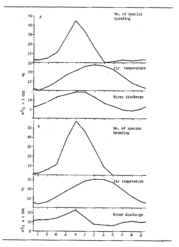
Figure 6.9 Number of fish species spawning in different months of the year compared with air temperature and river discharge in (A) the Danube river and (B) the Mississippi river
Where the highest temperatures of the year occur at the same time as low water some conflict between the two stimuli may occur. In the Okavango Delta spawning of most species takes place in the warmer months of the year, (September-March). This period coincides with the flood in the North basin of the swamp, but in most of the delta the flood occurs in the coldest part of the year and the fish breed during low water (Fox et al., 1976).
The factors which initiate maturation and stimulate breeding of floodplain fishes are elsewhere less clear and a number of factors have been implicated including changes in individual physical parameters such as temperature, conductivity or flow, as well as the assemblage of conditions that mark the beginning of the flood. It is probable that each species is affected by the various factors in different ways and that such external releasers are only effective when superimposed on an internal physiological rhythm of the fish. An illustration of the specificity of those conditions that induce spawning is Pimelodus maculatus of the Jaguari river. Basile-Martins et al. (1975) considered that maturation of this species started when temperatures reached 22°C and that a temperature of 25°C was needed for breeding to occur. However, temperature was not the only regulatory mechanism as a minimum increase in water level of 1 m over the low water level also seemed necessary to trigger spawning (Fig. 6.10). Changes in gonadosomatic index (GSI) where:
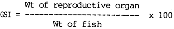
were also used to define breeding of Alestes baremoze in the Chari delta which coincides both with rising flood and increase in rainfall (Durand and Loubens, 1970), and in this species Paugy (1978) concluded that the high temperature attained during the dry season was necessary for maturation whereas the arrival of the flood triggered actual spawning. The relationship between endocrine activity, spawning, rainfall, temperature and daylength have been presented for the Indian catfish Heteropneustes fossilis (Viswanathan and Sundararaj, 1974). These three examples, together with other observations show the underlying similarity of timing of maturity and spawning. It is well known that many of the migratory characins and cyprinids will not spawn unless the flood materializes. As Bonetto (1975) has noted, individuals of Prochilodus platensis which are isolated in the floodplain lagoons do not mature when fish in the river channel do. Most Indian investigators agree that the major carps will not breed if the flooding associated with the monsoon fails (Parameswaran et al., 1970). Under these conditions, suitable inundated spawning grounds also have to be available for reproduction to be successfully concluded, although one cyprinid, Cirrhinus reba differs from this in that it can breed even at low water in the Cauvery and Bhavani rivers provided sexual readiness is induced by a short initial spate (Rao et al., 1972). According to Sidthimunka (1972) Probarbus jullieni shows similar behaviour in the Mekong system and Krykhtin (1975) reported that, while many food fishes from the river Amur bred only on the floodplain with rises in water level, some species (e.g., Elopichthys bambusa, Erythroculter sp. also reproduced when the water level did not rise. Indeed many phytophylic species in European rivers appear to have adapted to the modified conditions following channelization and flood control by spawning within the main channel rather than on the fringing flooded areas. However, in these species the main external factor regulating spawning seems to be temperature rather than flow.
Despite such exceptions it may be concluded that in the majority of total spawning species breeding is so timed that if floods are delayed or inadequate to trigger migration reproduction may fail in that year. Partial spawning species appear to be capable of breeding whenever suitable conditions are present and as has already been noted some such species breed throughout the year. Many others have longer and more diffuse breeding seasons, starting to breed in the river channel before the floods arrive and continuing with subsequent broods well into the flood season on the plain.
Maturation tends to be relatively rapid in river species. Most small tropical species are ready to spawn by the onset of the rainy season following their birth and have very short life cycles (Lowe-McConnell, 1967). Equivalent sized species in the temperate zone mature somewhat later, either during the first or more usually the second year of life. Larger species in both tropics and temperate zones often delay maturation until their third or fourth years and extreme examples such as Aspius aspius or Catastomus catastomus may not begin spawning until their fifth year. Species in unstable systems may respond to unfavourable circumstances by stunting and accelerating maturation within the first year of life. Such behaviour is typical of species of the genus Oreochromis (Dudley, 1976).
Hatching times of eggs are in most cases closely related to water temperatures and they differ considerably in any one species. For instance, eggs of Esox lucius which hatch in 12–14 days at 7–9°C hatch in 4–5 days at 17–20°C, and in brown trout incubation times of 148 days at 2°C are reduced to 27 days at 12°C (Table 6.9).
Figure 6.10 Gonadosomatic index (GSI) of Pimelodus maculatus in the river Jaguari compared with temperature (T°C), water level in river (m) and rainfall (mm³) for 1971–73. (After Basile Martins et al., 1975)
| Water temperature °C | Incubation time days |
|---|---|
| 2.0 | 148 |
| 3.6 | 118 |
| 4.7 | 97 |
| 6.0 | 77 |
| 7.8 | 60 |
| 10.0 | 41 |
| 11.0 | 35 |
| 12.0 | 27 |
Because of the cooler and less predictable thermal conditions temperate species have larger and more variable hatching times usually ranging from 5–10 days. In the tropics, with higher and more constant temperatures, hatching is rapid and in some fishes may occur within 16–24 hours of the eggs being laid. Such fast development has been noted particularly from open substratum spawners such as Hilsa ilisha (Pillay and Rosa, 1963), Labeo rohita (Kahn and Jhingran, 1975) and Labeo victorianus (Fryer and Whitehead, 1959). The eggs of some nest building species develop equally fast, although in mouthbrooders the eggs take longer to hatch (4–5 days) and the fry often stay with the parent for up to 2 weeks.
Exceptionally long hatching times are also common in some species. Many of the autumn or winter spawners of temperate rivers, such as Salmo trutta have development times of up to three months meaning that hatching usually occurs in early spring. Similarly the drought resistant eggs of Nothobranchius spp. may arrest development for over a year until favourable conditions prevail.
Several aspects of the flood regime can have an impact on breeding success or on the survival of fry, and thereby influence recruitment to the fish stock. That there are considerable differences in the numbers of young produced in various years is well known. Holden (1963) noted that some species were only represented by one year class in the Sokoto river. There were also great variations in the relative abundance of species, indicating year to year differences in breeding success. Non-migratory species were most abundant in one year (1955) due to a strong 1954 year class correlated with a good early rise of the river. The same factor obviously did not favour the migratory species. Holden also mentions the observations of Wimpenny (1934) on the Nile delta lake where heavy floods were followed by good recruitment giving a high density of fish. LoweMcConnell (1964 and 1967) noted large fluctuations in abundance of different species in different years, which she attributed to differential breeding success, short life cycles and rapid maturation. Here strong year classes of Serrasalmus nattereri and Prochilodus were found in different years.
In the Amur system, the yield of phytophilous species, which breed on the floodplain of the river, is also directly related to the flood regime. Year classes are usually weak in years of light flooding and strong when floods are heavy (Nikolsky, 1956). That a similar dependency between recruitment and flood regime exists in the Danube is indicated by the fluctuations in fish yield as a correlate of water level analysed by Holcik and Bastl (1977).
From fluctuations in the number of Oreochromis andersoni, O. macrochir, and Tilapia rendalli, Dudley (1972) deduced that there were seasonal changes in abundance. Furthermore, from differences in the abundance of Oreochromis juveniles he concluded that breeding success and recruitment to the stock was much better in those years having good floods. Later work on O. andersoni and O. macrochir indicated that spawning success might have been depressed by high dry season water levels. The reason advanced for this is that Oreochromis normally stunt under the severer conditions where drawdown is greater. The stunted fish mature and breed earlier than they would in years when the high volume of water retained allows fish to grow to their normal maturation size.
The extreme hydrological conditions of the Sahelian rivers during the 1970–1974 period have provided examples of the effects of failed floods on the recruitment of several fish species. In the Central Delta of the Niger, Dansoko (1975) and Dansoko et al. (1976) compared the biology of Hydrocynus brevis and H. forskahlii. The floodplain spawning H. brevis and the main channel spawning H. forskahlii give a useful contrast in that the effect of variability in the extent of flooding should be reflected more in one species that the other. This was confirmed by poor recruitment in H. brevis during the years when the flood failed. A similar succession of events happened in the Senegal river where recruitment of all freshwater fish was lacking in the poor flood years of 1968 and also in 1971 as exemplified by Citharinus citharus in Fig. 6.8. In the Chari river several species have disappeared following the sustained Sahelian drought which hindered breeding in the Yaeres floodplains as well as producing unfavourable conditions in the river channel and in Lake Chad. Larger species, Distichodus, Citharinus and Labeo and the migratory Alestes dentex and A. baremoze, declined drastically in abundance and were replaced by other species including Hemisynodontis membranaceus and Brachysynodontis batensoda. Oreochromis niloticus, because of its multiple spawning habit could rapidly recolonize the floodplains once more favourable conditions appeared, whereas in species such as Alestes, which are total spawners where the majority of the new recruits are produced by the second and third year classes, a failure of two floods in succession so weakened the stock that it appeared unable to recover especially in the face of continued heavy fishery (Carmouze et al., 1983).
Any consideration of mortality among river fishes is liable to be complex because of the interplay among the many causes of death. Two main groups of natural factors may be identified: (i) Density dependant factors whose rate is a function of the numbers of individuals of the species or of other species within a given space, and (ii) Density independant factors which usually are non-biotic and which originate in the changing physical and chemical characteristics of the river system. The two groups of factors are interrelated especially in rivers with fluctuating water regimes as changes in the volume of the living space constantly influence the density of the fish themselves. Equally the various density dependant factors can affect the rate at which others proceed; for instance having mortalities due to predation at one phase of the flood cycle can so reduce populations of prey species that their subsequent mortality through competition among themselves is considerably reduced. An indication of the linkages between some of these factors is shown in Fig. 6.11 for the fry and parr stages of stream dwelling salmonids.
Figure 6.11 Summary of factors which effect changes in numbers of stream dwelling salmonids during the fry and parr stages (from McFadden, 1969)
To the natural causes of mortality should be added fishing mortality. Attempts at separating natural and fishing mortalities in river fisheries are rare. In any case, because most techniques employed in artisanal river fisheries are themselves density dependant, the effects of removal of fish by fishing may significantly alter the rate at which they die from other causes.
Death due to stranding or isolation of fish in headwater streams, main channel pools or temporary water bodies on the floodplain is probably one of the major elements of natural mortality. Bonetto et al. (1969) estimated that some 40 000 t of fish are lost in this way from the Parana system, basing their estimate on the area of standing water on the plain (2 × 10⁶ ha²) and the standing stocks of 20 kg/ha as estimated from a small sample of them. This figure was greatly superior to the 10 000 t which were reported to have been caught by the fishery in 1967. There is no doubt that enormous quantities of fish are lost in this manner in most systems, and this apparent wastefulness has been widely remarked upon in the literature. Mortality through stranding is obviously closely related to the flood regime. It is not particularly prominent during the rising flood although temporarily recessions can leave fish isolated in pools and can destroy young fish in nests at the flood margin. More extensive flooding can raise the total number or biomass of fish in the system through improved reproductive success and growth making the whole community more sensitive to later contractions in the volume of the aquatic environment. The form of the falling flood would appear to be critical, as a more rapid draining of the plain would seem to give the fish less time to abandon their flood habitats and would increase the chances of their being isolated in unsuitable places. On the other hand there is a possibility that there might also be some favourable effects because of the stronger pattern of currents which may make the fish more responsive to such stimuli. However, the behaviour of fish during the return movement to the main channel has not been studied in any great detail and needs considerable work in the future. The duration of the dry season equally affects the proportion of the standing water that will disappear through evaporation or be rendered unsuitable for habitation by certain species. Presumably the longer and more severe the dry period, the greater the mortality due to this cause. The impact of stranding mortality on the dynamics of the community as a whole is difficult to assess. If all of the fish produced during one wet season were to enter the permanent standing water at the end of the flood, densities far surpassing the carrying capacity of the water might well result. This could give rise to a corresponding increase in density dependent mortality with a final survival not far different from that resulting when a proportion of the individuals are lost by stranding.
Deaths due to unfavourable hydrological conditions during the floods have been described from several systems. In the Kafue flats (Tait, 1967) and the Parana, these have been traced to the deoxygenation of the whole water column in lagoons when the lowering of the temperature and high winds cause the breakdown of stratification and sudden overturn. Similar cold spells have been the source of recorded mortalities in the Nile and in the Amazon, where they are known as “friagems”, Brinkmann and Santos, 1973). In the Amur river, winter kill conditions arise in years of poor low water flow when the main channel separates into a number of pools. These become deoxygenated causing heavy mortalities of adult fishes (Krykhtin, 1975). Heavy fish kills in pools within the channels of small stream or even major rivers produced by high temperature or deoxygenated conditions are also common especially in the tropics or in temperate zones where eutrophicated of polluted conditions prevail. Fish kills due to such causes are often spectacular in that large numbers of dead fish appear on the surface, but they generally seem to be highly localized in space and time.
Reduced survival of stream living species and of the young of upstream spawners can be anticipated in years of exceptionally heavy flooding. In such an eventuality the semi-pelagic eggs, juveniles and even the fish themselves could be swept downstream past the most favourable sites for their development. Similarly, fish may be lost to the community by the downstream drift of sudd islands in which they have taken refuge. These islands may eventually reach saline or other unsuitable waters where the fish die. In estuarine systems too, mortalities of freshwater fish have been observed when they have been carried out to sea by excessive currents.
Many of the species of fish inhabiting rivers are of small size and have life spans of one or at the most two years. Death in such fishes is possibly associated with stresses arising from spawning or from senescence. The mechanisms defining the life span of any species are, however, not well understood and many fish live for considerably longer periods in captivity than they would seem to do in their natural habitats.
Intraspecific or interspecific competition is obviously one of the main potential causes of density dependant mortality among species. Competition may be for food or, perhaps more commonly, for some other limiting resource such as shade, refuge sites or breeding sites. In some species, particularly redd cutting species such as salmonids, the phenomenon of overcutting, where one fish destroys the eggs of a previous spawner, increases at high population densities. Also demonstrated for salmonids is the exclusion of juveniles from feeding territories by incumbent fish at densities much above 5 fry/m² (Le Cren, 1965) resulting in a plateaux in population at about this level. Le Cren was able to obtain experimentally a linear relationship between the coefficient of mortality (%) and the logarithm of the numbers of Salmo trutta present in a stream. Such relationships indicate the extent to which direct intraspecific competition may affect populations as density increases.
Interspecific competition may also produce local differences in mortality rates, but in view of the continual co-survival of multi-speciate fish communities over long periods of time it obviously does not represent a major cause of mortality. Perhaps the most widespread interspecific contribution to mortality is that of predation. As has already been noted, the role of piscivorous predators in the community increases with stream order and predators form a particularly large proportion of the biomass in the potamon. Here mortality of small species and of the juveniles of larger species due to predation by fish is probably maximal during the draining of the floodplain after the flood peak has passed. Evidence presented in the section on feeding indicates that in many tropical rivers, predators do not feed extensively during the dry season. There is unfortunately no data on the intensity of predation during the rising floods. At this time cover for prey is maximal and the fish are probably dispersed widely over the plain. Nevertheless, the condition of the predators improves throughout this period indicating that they are feeding to a certain extent. The juveniles of most predatory species use alternative food resources during the earlier stages of the flood, but are already turning to a piscivorous habit as the flood nears its end. During the run-off phase the stomachs of most predators are full, and personal observations on the Oueme and Niger showed them to be typically packed with the juveniles of a wide range of species. Prey may include the young of the predators themselves whose non-specific feeding habits may lead them to cannibalism. Selection by length of prey is, however, much more widespread, and there would appear to be a relatively narrow size range at which different species are vulnerable to predation.
Predation by animals other than fish also appears to be at its highest during the period of the draining of the plain. Williams (1971) and Lowe-McConnell (1964), together with several other workers, have remarked particularly on the number of water birds preying on the fish stranded in floodplain depression or leaving the area by way of the channels.
Another possible contributor to total natural mortality is disease. This may become extremely important during the phase of high fish concentrations at the end of the dry season. A range of diseases infect salmonid and cyprinid species in temperate rivers. These are mostly associated with the high densities of fish attained in intensive fish culture but easily spread to the wild. There is little knowledge of the epidemiology of tropical fishes in their natural habitats, although Khalil (1971) recorded 215 genera of helminths, and Awachie et al. (1977) listed a range of bacteria, protozoa and Crustacea, all of which are parasitic on fish in African inland waters. According to Awachie et al. (1977) the lotic conditions in rivers are not favourable to heavy infestations with such parasites. However, large mortalities have been recorded from the various eleotrid species from the Sepik river in Papua New Guinea. These were traced to the bacterium Aeromonas hydrophila, the causative agent of dermal necrosis, and occured not only among species inhabiting the floodplain but also those of the headwater streams (Coates, 1984). A similar disease has been reported as spread throughout S.E. Asian rivers in the early 1980s. That reservoirs of infection are present among natural populations in rivers is also indicated by the rapidity with which a variety of diseases appear and spread through populations of ornamental fish after their capture. Much would appear to depend on the concentration of fish in the habitat and the swiftness of the current. In sheltered lentic environments the abundance of parasitic organisms increases. Such conditions are present in floodplain pools or isolated main stream pools in the dry season where the lack of current, warm temperatures and high population densities of fish favour the spread of infection. Likewise, parasitic infestations are readily discernable on nursery beaches where young Oreochromis and Tilapia congregate. Under crowded conditions too, there is a build up of toxic excretory products, mainly NH3 and N02 in the water. These themselves lead to gill or skin damage, which in conjunction with heavy parasite infestations can cause death.
The various factors contributing to total mortality tend to follow a similar pattern in fluctuating systems. Apart from deaths due to unfavourable conditions during rising floods, and the sweeping away of juvenile or small fish also during this time, most causes of death intensify as the flood cycle passes from wet to dry phase. Due to the fluctuating volume of the aquatic components of the river there is a range of ichthyomass that can be suported by it. Available evidence suggests that the maximum amount of fish is present during the flood and the minimum just before the onset of the next flood. This means that there is an overproduction of ichthyomass during the flood which persists throughout the period of falling water and which must be lost through total mortality during the dry season. It also implies that the amount of water remaining in the system during the dry season relative to the amount of water present during the wet, is one of the major factors determining mortality. Because there is an overproduction of ichthyomass during the wet season the biotic system can respond to differences in the amount of water during the dry season so as to assure maximum survival into the next year. What proportion of total mortality can be taken as fishing mortality without affecting this flexibility of response is one of the key questions in the dynamics of river fish communities and in the management of their stocks for fisheries.
Total mortality rates (Z) are derived from the formula
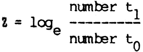
and represents loss from a habitat or component of the ecosystem by death from all sources including fishing, and the difference between immigration into emigration from the area under study. Obviously, the larger the area sampled to establish Nt and Nt0 relative to the size of the whole system, the more errors arising from immigration and emigration are liable to be reduced and the more Z tends to represent death rate. Only very few estimates have been made for species of fish inhabiting tropical rivers and these are given in Table 6.10. Values of Z are generally quite high in the early years of life (Z 4) but tend to drop during the later years (Z 1). This may be because the fish become less susceptible to predation as their size increases, and large species such as Colossoma have low mortality rates even when young although heavy fishing pressure continues on most species throughout their lives. In the extreme case of fishes whose life spans are very short, for instance the one to two years of many species of Barbus, cyprinodont or small mormyrid, values of Z, can be very high.
Comparison with mortality rates of fish from temperate rivers shows that, although survival is better initially in the temperate species (low mortality rates), their mortality rates tend to increase with age.
An accurate knowledge of mortality rates is essential to the calculation of production an animal communities, the lack of precise knowledge of this parameter for tropical riverine fish is a severe handicap in understanding the dynamics of such populations, however indications of mortality rate may be taken from Pauly's (1980) demonstration of the inverse relationship between mortality and asymptotic length in fishes.
The simple exponential model of mortality Nt = Noe-zt has been widely used to des cribe year to year mortality of fishes. If used to describe mortality patterns during one year it assumes stable environmental conditions such as these in reservoir rivers or canals and predicts maximum loss of numbers early in the period under consideration. Such a model, however, does not adequately describe mortalities within any one year in rivers with fluctuating hydrological regimes. To more accurately represent mortality patterns under such regimes Kapetsky (1974) suggested that the form of the mortality curve might be represented by rotating the curve for exponential decrease in number around its diagonal axis. This gives a curve of the form:
Nt = N0 - N0 exp - zT[(exp zt)-l]
where z is a weekly mortality coefficient, to is equivalent to the time of recruitment, t = time in weeks and T = 52 weeks. Such a curve gives a mortality rate which increases steadily throughout the year (Fig. 6.12). While not wholly satisfactory this model is a useful generalization for use in broader productivity models. The seasonal patterns of mortality described above indicate very little mortality during the wet season and increased mortality as the year progresses. The majority of causes of death: predation, fishing, disease, hostile environments, etc., would seem to be density linked, and for this reason Welcomme and Hagborg (1977) reduced the number of fish in a similated floodplain population by inserting a density dependent mortality parameter in the simple exponential model:
Nt+1 = Nt exp - (exp zM)
| Species | River | Year | Author | ||||||||
|---|---|---|---|---|---|---|---|---|---|---|---|
| 1 | 2 | 3 | 4 | 5 | 6 | 7 | 8 | 9 | |||
| TROPICAL | |||||||||||
| Polypterus senegalus | Chari | 0.54 | 0.53 | Daget and Ecoutin, 1976 | |||||||
| Brycinus leuciscus | Niger | 1.20 | Daget and Ecoutin, 1976 | ||||||||
| Hydrocynus brevis | Niger | 3.08 | 0.98 | Dansoko, 1975 | |||||||
| Hydrocynus forskahlii | Niger | 2.49 | 2.67 | Dansoki, 1975 | |||||||
| Oreochromis andersoni | Kafue | 2.47 | 0.65 | 0.65 | 0.65 | 0.65 | 1.70 | 0.58 | 0.58 | Kapetsky,1974a | |
| Oreochromis macrochir | Kafue | 3.98 | 0.70 | 0.70 | 0.70 | 0.70 | 0.70 | Kapetsky, 1974a | |||
| Tilapia rendalli | Kafue | 4.61 | 1.40 | 1.40 | 1.40 | 1.40 | Kapetsky, 1974a | ||||
| Serranochromis angusticeps | Kafue | 3.12 | 2.20 | Kapetsky, 1974a | |||||||
| Hepsetus odoe | Kafue | 2.74 | 1.84 | 1.84 | 1.84 | Kapetsky, 1974a | |||||
| Total community* | Bandama | 2.67 | Daget et al., 1973 | ||||||||
| Colossoma macropomum | Amazon | 0.45 | 0.45 | Petrere, 1983 | |||||||
| TEMPERATE | |||||||||||
| Salmo trutta | Bere stream | 2.10 | 1.34 | 1.81 | Mann, 1971 | ||||||
| Cottus gobio | Bere stream | 1.66 | 1.33 | Mann, 1971 | |||||||
| Rutilus rutilus | Thames | 0.42 | 0.42 | 0.68 | 0.70 | 0.92 | 1.00 | 1.26 | 1.86 | Mann, 1971 | |
| Rutilus rutilus | Danube | 0.69 | 0.98 | 0.65 | 0.70 | 0.56 | 0.61 | 0.68 | 0.75 | Chitrava- divelu, 1972 | |
| Alburnus alburnus | Thames | 1.29 | 1.29 | 1.29 | 3.90 | 4.80 | 4.10 | Mann, 1971 | |||
| Danube | 0.88 | 0.86 | 0.82 | 0.84 | 0.73 | 0.63 | Chitrava- divelu, 1972 | ||||
| Leuciscus leuciscus | Thames | 0.60 | 0.60 | 0.60 | 0.60 | 0.56 | 1.15 | 1.28 | 1.46 | Mann, 1971 | |
| Perca fluviatilis | Thames | 0.98 | 0.98 | 0.98 | 1.61 | 1.49 | 1.39 | 1.45 | 1.47 | Mann, 1971 | |
| Gobio gobio | Thames | 0.88 | 0.88 | 0.88 | 0.88 | 2.52 | 4.24 | Mann, 1971 | |||
* Dominant species Labeo coubie and Alestes rutilus
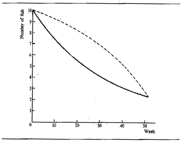
Figure 6.12 Changes in number of fish in one age group over 52 weeks as predicted by a simple exponential model (—) and Kapetsky's (1974) floodplain model (-----): z = 1.5
In this simulation z was obtained from a mortality coefficient characteristic of selected floodplain fish species; M was calculated from a formula of the form M = aBx where B is the weight per unit volume of the fish in the system. M was adjusted to unity at a preselected biomass typical of a floodplain system, producing slower mortality rates when densities fell below the biomass and increased mortality rates at greater densities. The results of such a simulation are shown in Fig. 6.13.
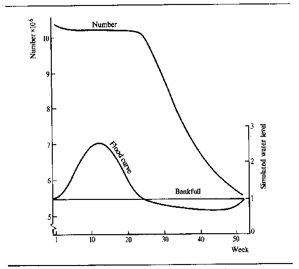
Figure 6.13 Changes in the number of fish in one age group over 52 weeks assuming recruitment at the start of week 1 when generated by the simulation of Welcomme and Hagborg (1977). Also shown are the water levels used in the simulation.
Estimates of ichthyomass or standing stock are available from many rivers and sufficient information exists to permit a preliminary comparison between temperate and tropical waters. Standing stock estimates are usually made by one or more of three basic techniques: multiple fishing to the exhaustion of the stock, mark and recapture experiments, and poisoning a sample area with piscicides. The assessment of the total fish population by these methods is not wholly reliable due to sampling errors of various kinds, but the combination of several methods and the taking of samples over large areas improves the reliability of the estimate.
The density of the population present in rivers with fluctuating water regimes depends much on the amount of water present at the time of sampling. Population densities (ichthyomass per unit area) are generally higher during low water when the fish are concentrated together than at high water when they are dispersed, even though the total weight of fish in the system may be larger during the floods. Furthermore, the degree of exploitation affects the standing stock with probable reduction in mean ichthyomass as fishing pressure increases. As many water courses are very heavily fished, particularly in the tropics, the values of ichthyomass might be expected to be lower than they would be in a virgin or unexploited stock. Comparison between different systems is therefore difficult and can only legitimately be made on the basis of samples taken during the same phase of the flood cycle and taking into account the state of exploitation of the stock.
Differences in standing stock in the main channel may be correlated with ecological parameters such as slope. In general there is a progressive increase in ichthyomass as one moves downstream, as for instance in the Luanza River, Zaire where Malaisse (1969 and 1976) found 1.3 kg/km, 26.1 kg/km and 31.7 kg/km in successive downstream reaches (see also Table 6.11). Much of this increase may be traced to the widening of the river channel downstream, hence standing stock (Ichthyomass/unit area) may not increase at such a rate. However, where the fall line of the river does increase lower ichthomasses are present, as in the case of the Kaloma River where a reach with greater slope had an ichthyomass of 7 kg/km and was intermediate between an upstream reach with 21 kg/km and a downstream reach with 91 kg/km (Balon and Coche, 1974). This implies that there may be a trend to increase in overall productivity along the river channel with higher standing stocks, downstream although much more work is needed to clarify the ecology of small tropical streams.
In most rivers, flows are too swift for accurate samples to be taken during the floods in the main channel. Consequently most estimates have to be made during low water. It was assumed by the University of Michigan et al. (1971) that during the floods the ichthyomass in the Kafue river would not differ significantly from that of the open water areas of the floodplain where, on the basis of repeated fishing with seine nets and on rotenone samples in the open waters, an ichthyomass of 337 kg/ha was established. Samples taken in the channel at low water showed the standing stock to be less, 204 kg/ha. In the light of work by Kapetsky (1974) this dry season estimate may be somewhat low as he found the standing stock of the five main commercial species to be very different for three separate reaches of the Kafue river, at 106.5 +29.21; 576.7 ± 129.2 and 386.6 ± 63.9 kg/ha respectively. The differences in standing stocks were attributed to differences in fishing intensity in the various reaches. The discrepancy betweeen the mean 348.2 ± 59.5 kg/ha and the 204 kg/ha found by the University of Michigan could be explained in part by the reduction in water volume by a factor of 0.7 between the two sets of samples, but because the University estimate is based on all fish species, the actual difference between the two estimates is most probably greater than it appears.
In the Chari river, Loubens (1969) carried out an estimate of standing stock in a 360 m² pool left in the main channel at low water obtaining 15 138 fish/ha weighing 861 kg/ha. More comprehensive results were quoted by Daget et al. (1973), whose rotenone sampling at two sites in the Bandama river enabled the evaluation of changes occurring in the dry season. These were reduced into the formulae: for the reduction in number (dj) with time in days (j). At one site, numbers were reduced from 3 417 fish/ha on 31 January to 1 411 fish/ha on 30 May, and biomass fell from 125 kg/ha to 50 kg/ha in the same period. At the other site, 2 271 fish/ha on 31 January decreased to 996 fish/ha on 2 August, a loss of biomass of 144 kg/ha from 257 kg/ha to 113 kg/ha. The lower estimates of standing stock obtained from the Mekong by Sidthimunka (1970) of 6.0 and 7.4 kg/ha were attributed to difficulties in sampling and one sample from the Mong tributary of the river gave the much higher value of 137.4 km/ha. Other small rivers in Thailand have been recorded with very similar levels of standing stock, 118, 186 and 81 kg/ha for the Bori Pat, Lami Pi and Muak Lek rivers respectively (Geisler et al., 1979). Bishop (1973) also calculated an ichthyomass of 179 kg/ha in the small black water Gombak river in Malaysia although that estimate was arrived at by assuming only 20% efficiency with electro fishing gear applied to catches equivalent to about 38 kg/ha.
Log dj = 1.63292 - 0.003202j and Log dj = 1.67286 - 0.003166j
Unpublished fishery studies relating to the lower Mekong basin, prepared under the auspices of the Mekong Committee present values of 60 kg/ha for the upstream Mun river tributary to the Mekong, and 91.9 ± 51.7 kg/ha for 11 other tributaries. The value of 60 kg/ha for the Mun river is a mean of several estimates which fall from 120 kg/ha at low water to 5 kg/ha during the rising flood. The progressive drop of ichthyomass per unit area is attributed to the dispersal of the stock with increasing volume of water. Downstream in the main inundation zone the riverine standing crop was estimated at 135 kg/ha, but as this and the other values quoted are derived from capture fisheries the authors consider them to be low and they probably exclude the first year fish which, as has been shown, contribute the major part of the ichthyomass. The basic productivity of the water may also effect the standing stock, especially in exploited populations. In black water rivers relatively low values of ichthyomass may be anticipated, such as the 88.7 ± 75.7 kg/ha from the Baram River (Watson and Balon, 1983), although no correlation between nutrient status and standing stock was found by Geisler et al. (1979) in Amazonian rivers and analysis of standing stock against conductivity yields no significant results. Considerably more data is needed from black waters in order to more fully understand their ecology.
Much work has been done on the fish populations of temperate rivers to determine their ichthyomass (Table 6.11). For example, Mann (1965) found a total ichthyomass of 659 kg/ha in the river Thames, a value which he considered high for temperate rivers, although Backiel (1971) estimated that total ichthyomass in the Vistula river may be between 200 and 1 100 kg/ha. In Belgian rivers of various sizes, Timmermans (1961) and Huet and Timmermans (1963) found between 130 and 300 kg of fish/ha by electrofishing. Philippart (1978) found that the total ichthyomass in the river Ourthe corresponded to 315 kg/ha, or approximately 900 kg/km. Within this mean biomass fluctuated following various factors such as temperature or depth of water but the main correlate was with channel width according to the formula:
Ichthyomass = 6.9569 x 1.8456 (r = 0.919)
Detailed analysis of 40 Belgian rivers shows the main biomass to be 197.8 ± 137.8 kg/ha although potamon reaches such as the Ourthe or Semois Rivers range between 250–350 kg/ha. An inverse relationship was established by Timmermans and by Cuinat (1971) for French rivers:
posit that small rivers with high slope have a larger biomass per unit area, at least in Europe. Philippart (1978a) proposed a modified model:
B = -295 + 0.19A + 5.72T+17.58S +16.8W
where A = alkalinity; T = mean temperature; S = mean slope and W = mean width based on the set of Belgian rivers. Similar values have been obtained from temperate rivers other than those of Europe. For example, the Horokiwi stream in New Zealand supported up to 311 kg/ha of fish (Allen, 1951) and ichthyomass in trout streams in North America may reach 471 kg/ha (McFadden and Cooper, 1962). Swingle (1954) recorded 143 kg/ha from deep parts of the Coosa river and 154 kg/ha for shallow areas. Ichthyomass in deep parts of other large Alabama rivers varied from 51.2 to 1 730 kg/ha, this latter being attained in the Tenson river which had a particularly wide floodplain. Further to the North, Mahon et al. (1979) found 11 126-74 765 individuals/ha, equivalent to 32.4 to 190 kg/ha for the Speed river Ontario.
This brief survey of standing stocks from streams all over the world indicates a wide range of values at all latitudes. It is perhaps surprising, however, to find that there is little basis for any supposed higher carrying capacity in the tropics. In fact values of between 100 and 600 kg/ha are common in all continental areas.
Secondary channels and blind river arms, which have many of the characteristics of floodplain standing waters but remain connected to the main channel for most of the year, are richer habitats than the main river.
Perhaps the most detailed studies of fish populations of river backwaters come from the Danube. Bastl et al. (1969), Holcik (1972), Holcik and Bastl (1973 and 1976) and Chitravadivelu (1974) have investigated the Biskupicke, Zofin and Vojka branches using mark-recapture and repeated catching methods. Their work led to the generalization that ichthyomass varies between 300 and 500 kg/ha. About 20 species were present although species number varied with the area of the arm. Population densities were high in the summer when fish took refuge in the side arm from the current in the main channel. In the autumn the ichthyomass dropped as larger fish disappeared from the shallower waters. Very low values, often below 100 kg/ha were associated with unusually strong flooding which dispersed the population, or with pollution which was especially common in same side arms of the Danube. A similar ichthyomass has been recorded from the Poltruba arm of the Elbe, where Oliva (1960) found a population density of Rutilus rutilus and Alburnus alburnus of 222.3 kg/ha using rotenone. As this was obtained from only two species the total ichthyomass was presumably somewhat higher. As many as 22 350 fish/ha were found in a secondary arm of the Chari by Loubens (1969) although 98 percent of these were small fish of less than 10 cm length. By contrast, 96 percent of the 2 150 kg/ha were contributed by the few fish larger than this length. The same backwater had 5 616 kg of fish/ha at the end of one flood which had fallen to 1 600 kg/ha two months later. A fourth sample from the same area a year later, only yielded 369 kg/ha, indicating the year to year variability that can be expected in the same body of water. Another backwater of the Chari gave an estimate of 2 166 kg/ha from an area of 6 000 m². In the Bandama, Daget et al. (1973) showed that population densities can increase in such backwaters. Contrary to the trends shown in the main channel, the number of fish in a minor river arm increased from 1 408 individuals/ha to 3 311 individuals/ha in June. This corresponded to an increase in weight from 149 kg/ha in March to 350 kg/ha in June. These figures, coupled with those for the main river, indicated that there is some movement during the dry season from the open pools of the main river into the more shaded habitats of the backwaters. Sidthimunka's (1970) figure of 219.8 kg/ha for a backwater to the main stream of the Mekong was also considerably higher than the estimates from the main river itself, although the Mekong studies figure of 125 kg/ha for a non-flowing backwater is similar to that in the main river. In the large Alabama Tombigbee river the ichthyomass in a backwater sampled by Swingle (1954) was much higher at 2 084 kg/ha, than either deep or shallow areas of the main stream with 457 and 570 kg/ha respectively.
Populations of fish in the floodplain lakes of the Danube are of similar densities to those of the backwaters. Balon (1967) in his sample of 13 water bodies, found between 335 to 318 632 fish/ha. The composition of the population varied considerably from one sample to another. The ichthyomass also had a wide range of variability; 230.4± 277.6 kg/ha. It was lowest during high water (136 ± 127 kg/ha in July) and highest during low water (480 ± 334 kg/ha). Other observations from seasonal water bodies of the Danube floodplain by Holcik et al. (1981) gave a mean of 366.7 ± 293.6 kg/ha. In the Russian Nyamunas river the floodplain is inundated by the spring floods which bring large quantities of fish into the oxbows and artificial channels. These are isolated during the summer and Gaygalas and Blatneve (1971) estimated that about 200 kg/ha of fish remained in the autumn. As about twice this number were caught by anglers the total spring biomass was probably closer to 500 kg/ha. The floodplain pools of the Canadian Irvine Creek System described by Halek and Balon (1983) supported standing stocks of 132.6 ± 57.7 kg/ha. Much of the variation between pools was attributed to the duration of the connection between the pools and the main river. Pools in which this connection persisted for some time had greater density of young of the year fish and hence higher mean biomass.
In tropical rivers standing stocks of floodplain pools tend to be somewhat higher although on some floodplains, such as the Magdalena and Mekong, there is a considerable movement out of the depressions toward the main river channel which may account for the low values obtained from such system. Table 6.11 summarizes the dry season ichthyomass from the standing waters of a sample of tropical rivers. Ichthyomass apparently varies according to a number of factors. As with other parts of the aquatic system, population densities are normally greater during the dry season. Thus when Kapetsky et al. (1976) estimated a minimum biomass of between 0.23 and 251 kg/ha (mean 55.7 kg/ha) as being presen t in the open water and between 20 and 232 kg/ha (mean 79.8 kg/ha) in the bay areas of the cienagas of the Magdalena floodplain he also found a good negative correlation between the population density and the water level in the cienagas. Strangely enough, whilst the University of Michigan et al. (1971) also found population densities to be higher in the open waters of the lagoons of the Kafue river during the dry season (426 kg/ha) than during the floods (337 kg/ha), vegetated areas showed the opposite tendency and very high concentrations of fish (up to 2 682 kg/ha) were present in such areas at high water. High densities of fish under floating vegetation seem to be comparably rare, however, and permanent swamps, particularly those under papyrus, are notorious for the poverty of their fish communities. This situation may change temporarily during the flood when currents can oxygenate the water column under the plants. The University of Michigan study also indicated the loss of ichthyomass during the dry season when in one pool an initial standing stock of 2 693 kg/ha diminished by 75% to 684 kg/ha in three months. In a second pool a similar decline from 3 306 to 501 kg/ha occurred in 10 weeks, although in this case the pool was connected to the river for part of the time and emigration might have occurred. Bonetto (1980a) studied a population of Prochilodus platensis which colonized the Laguna Gonzalez when it was flooded by the Riachuelo River in 1971/72. The lagoon subsequently remained isolated from the river and he was thus able to trace a single year class through a number of years by extrapolation from marck-recapture experiments. The isolation of the population from other year classes of Prochilodus undoubtedly gives a rather distorted picture of what happens in more normal lagoons. At the time of separation from the river the fish were probaly about 1 year old and, perhaps because of the limitation or food availability, the fish grew to a relatively small terminal length of 36 cm, as opposed to 60 cm in lagoons connected to the river. The standing stock increased from 232 kg/ha in the first year to 351 kg/ha in the second and decreased thereafter to 199 kg/ha in 1976 when observations ceased.
The form of the lagoon and the nature of the bottom may also influence ichthyomass. In the Senegal river, long narrow pools formed from isolated drainage channels supported a much higher standing stock than round depression pools, 205 ± 155 kg/ha as against 13 ± 6 kg/ha (Reizer, 1974). In the Sokoto, Holden's (1963) analysis shows that a greater proportion of fish preferred intermediate sand/mud bottoms (1 012 kg/ha) as opposed to sand (785 kg/ha) or mud (233 kg/ha).
Differences in standing stock have been related to the degree of organic fertilization of the water body by Fox (1976). His estimates for small uneriched pools in the southern Okavango delta showed between 100–200 kg/ha to be usual, whereas a highly enriched peripheral lagoon had the highest estimate of 700 kg/ha. While this evidence is far from conclusive due to the small sample size it would appear reasonable that eutrophicated waters should support higher densities of fish relative to those less rich in nutrients. Nutrient poor black waters on the other hand, appear to support lower standing stocks. For example, eight floodplain pools from the Rio Pacaya and Rio Saniria tributaries of the Peruvian Amazon gave 89.6 ± 37.1 kg/ha (Montreuil pers.comm.). However, there is still insufficient data available to attempt drawing some relationship between nutrient content and standing stock of fish in rivers.
| River | Size of sample | Estimated ichthyomass kg/ha | Author |
|---|---|---|---|
| Apure | 1 | 982 | Mago-Leccia, 1970 |
| Candaba | - | 500–700 | Delmendo, 1969 |
| Chari | 2 | 701–2 166 | Loubens, 1969 |
| Kafue | 8 | 444 | University of Michigan et al., 1971 |
| Magdalena | 28 | 122 | Kapetsky et al., 1977 |
| Mekong | 1 | 63 | Sidthimunka, 1970 |
| 390 | Mekong Fish. Studies (pers.comm.) | ||
| Mogi Guassu | 1 | 313 | Gomez and Montiero, 1955 |
| Nile Sudd | 2 | 306–433 | Mefit-Babtie, 1983 |
| Okavango | 2 | 200–700 | Fox, 1976 |
| Oueme | 68 | 1 835±825 | FAO/UN, 1971 |
| Parana | |||
Temporary lakes | 18 | 959±1 512 | Bonetto, 1976 |
Permanent lakes | 4 | 766±348 | |
| Sabaki | 1 | 786 | Whitehead, 1960 |
| Senegal | 8 | 110±144 | Reizer, 1974 |
| Sokoto | 25 | 661±557 | Holden, 1963 |
Standing stocks may also be influenced by the preceding flood history of the river, a topic treated in more detail under “Catch”. An example of such variability comes from the Atchafalaya distributary of the lower Mississippi where Bryan and Sabins (1979) recorded a lowering of standing crop of 795 kg ha in 1977 from 904 kg ha in 1975–76. The higher estimate comes from years preceded by good spring floods (1973–75) whereas the lower estimate comes from years preceded by poor floods (1976–77).
Studies analysing the contribution of the various components of a riverine system to the total standing stock are rare. However, one such study was carried out by the University of Michigan et al., (1971) who extrapolated rather widely from a limited number of samples of four different habitats of the Kafue river and floodplain. Their results are shown in Table 6.12.
A similar analysis was carried out by Holcik et al. (1981) for the Middle reaches of the Danube river with results as shown in Table 6.13.
| Area (ha²) | Ichthyomass (kg/ha) | Total ichthyomass (t) | |
|---|---|---|---|
| High water | |||
Open water lagoon | 126 000 | 337 | 42 462 |
Vegetated lagoon | 16 000 | 2 682 | 42 912 |
Grass marsh | 136 000 | 64 | 8 704 |
River channel | 5 300 | 337 | 1 786 |
Total | 283 300 | 338.4 | 95 864 |
| Low water | |||
River channel | 4 800 | 204 | 959 |
Open water lagoon | 113 000 | 426 | 48 138 |
Vegetated lagoon | 14 000 | 592 | 8 288 |
Total | 131 800 | 435.6 | 57 405 |
| Area (ha²) | Ichthyomass (kg/ha) | Total ichthyomass (t) | |
|---|---|---|---|
| Main channel | 7 936.9 | 35.0 | 277.8 |
| Backwaters | |||
Czechoslovak bank | 1 777.9 | 350.0 | 622.3 |
Hungarian bank | 1 336.0 | 400.0 | 534.4 |
Both banks | 3 113.9 | 371.5 | 1 156.5 |
Total | 11 050.8 | 129.76 | 1 434.3 |
A general estimate of ichthyomass has also been made for Atchafalaya river Louisiana from samples both in the mian channel and some floodplain lakes. Here a mean standing crop equivalaent to 860 kg/ha was calculated for the lower part of the basin and 555 kg/ha for the upper part (Bryan and Sabins, 1979).
Production can be defined as the total elaboration of fish tissue during any specified period, including gonadial products and material formed by individuals which do not survive to the end of the period (Ivlev, 1966). Standing stock and production estimates for a number of rivers are given in Table 6.14. Estimates of production range from a maximum of 2 000 kg/ha/yr in the Thames to as little as 16.2 kg/ha/yr in the Speed River but have a mean of 218.6±335.6 kg/ha/yr. Several factors may influence production among which the latitude, the basic productivity of the waters and the age structure of the population are perhaps the most important.
| River | Country | Biomass kg/ha | Production kg/ha/yr | P:B | Authority |
|---|---|---|---|---|---|
| Amazon Manaus | Brazil | 1600.0 | 2800.0 | 1.75 | Bayley (1983) |
| Thames | |||||
| (0+fish) | UK | 1315.0 | 2000.0 | 1.52 | Mann (1972) |
| (1+fish) | UK | 659.0 | 426.0 | 0.65 | Mann (1965) |
| Hinaki | N. Zealand | 880.8 | 735.4 | 0.82 | Hopkins (1971) |
| Kafue | Zambia | 520.0 | 618.0 | 1.19 | Kapetsky (1974) |
| Ellis | Canada | 376.0 | 375.4 | 1.0 | Mahon (1981) |
| Warkosc | Poland | 307.5 | 161.4 | 0.5 | Mahon (1981) |
| Carrol | Canada | 274.8 | 280.3 | 1.0 | Mahon (1981) |
| Hopewell | Canada | 228.4 | 263.5 | 1.0 | Mahon (1981) |
| Hinau II | N. Zealand | 217.7 | 241.7 | 1.11 | Hopkins (1971) |
| Lemki | USA | 212.0 | 136.0 | 0.64 | Goodnight and Bjornn (1971) |
| Jaruma | Spain | 178–221 | 221–583 | 1.2–2.6 | Lobon-Cervia and Penczak (1984) |
| Tarrant | UK | 198.0 | 596.0 | 3.01 | Mann (1971) |
| Kejin | Borneo | 173.1 | 261.5 | 1.50 | Watson and Balon (1984) |
| Bere | UK | 161.7 | 270.0 | 1.69 | Mann (1971) |
| Irvine | Canada | 149.9 | 226.4 | 1.50 | Mahon (1981) |
| Hall | UK | 129.0 | 52.0 | 0.40 | LeCren (1969) |
| Swann | Canada | 124.4 | 174.5 | 1.40 | Mahon (1981) |
| Struga | Poland | 111.2 | 110.3 | 1.0 | Mahon (1981) |
| Deer | USA | 84.7 | 160.0 | 1.89 | Chapman (1965) |
| Utrata | Poland | 84.5 | 289.3 | 3.4 | Penczak (1981) |
| Big Springs | USA | 84.2 | 118.0 | 1.4 | Goodnight and Bjornn (1971) |
| Mesta | Bulgaria | 80+82 | 80.0 | 1.0 | Penczak et al. (1984) |
| Dockens | UK | 75.0 | 140.0 | 1.87 | Mann (1971) |
| Clemons Fork | |||||
| (3rd 0) | USA | 71.5 | 77.2 | 1.08 | Lotrich (1973) |
| Kejin | Borneo | 71.0 | 98.3 | 1.4 | Watson and Balon (1984) |
| Clemons Fork | |||||
| (2nd 0) | USA | 63.6 | 105.5 | 1.66 | Lotrich (1973) |
| Appletreeworth | UK | 62.0 | 30.0 | 0.48 | LeCren (1969) |
| Black Brows | UK | 59.0 | 100.0 | 1.69 | LeCren (1969) |
| Clemons Fork | |||||
| (1st 0) | USA | 54.9 | 83.5 | 1.52 | Lotrich (1973) |
| Bobrza | Poland | 50.2 | 83.4 | 1.7 | Mahon (1981) |
| Needle Branch | USA | 45.9 | 90.0 | 1.96 | Chapman (1965) |
| Zalewka | Poland | 43.9 | 54.0 | 1.23 | Penczak (1981) |
| Kaka | Borneo | 38.5 | 47.5 | 1.2 | Watson and Balon (1984) |
| Wolborka | Poland | 37.4 | 35.3 | 0.94 | Penczak et al. (1982) |
| Speed (3rd Order) | Canada | 32.3 | 54.0 | 1.67 | Mahon et al. (1979) |
| Lava | Borneo | 30.5 | 39.3 | 1.3 | Watson and Balon (1984) |
| Payau | Borneo | 27.1 | 31.2 | 1.2 | Watson and Balon (1984) |
| Lawa | Borneo | 21.3 | 33.3 | 1.6 | Watson and Balon (1984) |
| Bulu | Borneo | 21.5 | 26.0 | 1.2 | Watson and Balon (1984) |
| Hinau I | N. Zealand | 19.6 | 42.8 | 2.18 | Hopkins (1971) |
| Speed (4th Order) | Canada | 7.0 | 16.2 | 2.31 | Mahon et al. (1979) |
It is commonly held that tropical waters are more productive than their temperate counterparts, and in lakes this undoubtedly appears to be the case. Unfortunately few observations exist on the productivity of tropical waters but those that do exist give little support to this contention. In fact the range, mean and standard deviation of standing stocks of 17 tropical rivers, 21.4 (154.4±198.7) 861 kg/ha/yr falls entirely within those of standing stocks for 26 temperate rivers, 7.0 (205.0±300.3) 1315 kg/ha/yr.
There is as yet equally little evidence for the lower productivity of rivers with lower ionic content, partly because so many other factors appear to influence the characteristics of the stock. However, in the tropics Watson and Balon's (1984) figure for black water streams from Borneo (conductivity >50 μmhos) is decidedly lower at 179.9 kg/ha/yr than Kapetsky's (1974) estimate of 678 kg/ha/yr for the richer Kafue (conductivity 130 – 320 μ mhos).
The influence of the proportion of juveniles in the stock is much clearer and Table 6.15 summarizes the percentage of total productivity contributed by various year classes in some fish species.
| Species | Percentage products by year class | Author | ||||
|---|---|---|---|---|---|---|
| 0+ | I | II | III | IV+ | ||
| Cottus cognatus | 65.1 | 20.0 | 12.2 | 2.5 | 0.2 | Petrovsky and Waters, 1975 |
| Salvelinus fontinalis | 40.8 | 41.0 | 14.7 | 3.1 | 0.4 | Dept. of Natural Resources, 1974 |
| Alburnus alburnus | 46.2 | 10.1 | 20.7 | 17.0 | 5.9 | Matthews, 1971 |
| Coltus gobio | 32.0 | 18.0 | 27.0 | 20.0 | 3.0 | Matthews, 1971 |
| Oreochromis andersoni | 61.2 | 22.8 | 12.2 | 2.2 | 1.6 | Kapetsky, 1974 |
| Oreochromis macrochir | 46.4 | 26.3 | 12.7 | 7.6 | 7.0 | Kapetsky, 1974 |
Theoretically there should be a smooth relationship such as that shown by S. fontinalis or C. cognatus where data was averaged over several years, but differences in year class strength due to differential success in recruitment, such as is shown by A. alburnus or R. rutilus may cause variations in overall productivity from year to year. Because of the great significance of juvenile fish to the total productivity, the efficiency of sampling for the younger year classes is of great importance and differences in population estimates may arise according to the degree to which the smaller fish are included in the sample. That year to year variations do occur in some systems is a matter of record but others show a remarkable constancy in productivity despite considerable changes in biomass. For example, the production of Salvelinus fontinalis varied by less than 20% around a mean of 117 kg/ha over 11 years of sampling in Lawrence Creek, Wisconsin. During the same period the biomass underwent almost threefold fluctuations from 13.5 to 99 kg/ha. This means that the efficiency of production was in this case strongly density dependent and a regression of P/B against biomass gave a significantly high correlation coefficient (Dept. of Natural Resources, 1974). From Table 6.14 it may be seen that, whereas standing stocks tend to be lower in lower order streams than in those of higher order, the productivity tends to increase resulting in higher P/B ratios. This high productivity of the rithron, especially in the riffles, may be accounted for in part by the larger numbers of juvenile fish in such areas (Schlosser, 1982). Production/Biomass ratios are generally useful indicators of the rapidity of turnover of biomass and, while productivity is strongly correlated to standing stock: variations do occur for a variety of reasons. As mentioned above the population density may influence the rate of production as also might the proportion of juvenile fish in the stock and a further factor that has been implicated is species composition. This latter may operate in two ways, firstly by the longevity of the species and secondly by its trophic status. The contention that short lived species have greater productivities (Leveque et al., 1977) can not be verified from the present data set, although it is to be anticipated that communities composed of small short lived species will have greater productions than communities of larger species inhabiting the same body of water. For similar reasons it may be supposed that predatory species, partly because of their generally large size and partly because of their position in the food chain, would have relatively lower productivities. In this case the mean value for P/B for 13 observations on 7 predatory species was much lower at 0.54±0.16 than the value of 1.2±0.5 for 95 observations on 37 species of all trophic categories and from both tropical and temperate waters. The difficulties inherent in this type of analysis are illustrated by the very wide range of P/B values obtained for some species; S. fontinalis, for instance, have been recorded as having ratios as low as 0.4 (LeCren, 1969) and as high as 3.0 (Mann, 1971).
P = 3.3 + 1.2 B (r² = 0.85 for the data listed in Table 6.14)
Several approaches have been used to study and estimate standing stocks in rivers. These vary according to the type of river in question, mainly because of difference in the ease with which various kinds of waters can be sampled. In general the difficulties of sampling large streams, usually defined as any water deeper than wading depth, and the large numbers of watercourses dictate the use of some type of predictive model, usually an index. Obviously such models have to be based on a certain number of estimates from the field and have to be verified from time to time in actual rivers. A second approach is through simulations based on theoretical concepts of the ecology of the fish community.
Simple models based upon environmental characteristicsSeveral attempts have been made at relating some characteristic of the fish community to the environment in which it lives. Usually such models or indices have been derived for practical purposes of fisheries management and it is not always clear exactly what is being predicted. For example, models will often claim to predict production when it is in fact catch that is meant and there is therefore some overlap between models dealt with in this section and those described in the section on appraisal of catch.
During their studies on the fishery resources of the rivers of Belgium and Northern France Leger, and later Huet, were able to formulate some generalizations as to the zonification of the running waters of temperate Europe. Arising from this Huet (1949 and 1964) proposed a simple model:
P = BLK
to assess the approximate inchthyomass available for exploitation in temperate rivers. In this model P = annual productivity (or harvest) of the water in kg/km of river, L = average width of the river, B = 'biogenic capacity' and K = coefficient of productivity. Values between 1 and 10 are assigned to B according to the amount of fish food (benthos) available. The coefficient K is the sum of K1, K2 and K3 where the value of K1 is derived from mean annual temperature, K2 depends on the acidity of the water and K3 summarizes the type of fish population.
This original method was modified by Lassleben (1977) for the assessment of fish catch from the German stretch of the Danube (Kolbing, 1978). In this case fish catch (C) for a section of river is determined as:
C = BK 10 kg/ha/yr
where B and the various components of K are as above except for K3 whose value may be derived from a simple equation establishing the proportion of each type of species present. This method has given good results in north Temperate streams and was extended to larger rivers such as the Danube by Holcik (1979) using the simple percentage of rheophilic and limnophilic species. The biogenic capacity of the river may be assessed using the biomass of benthic invertebrates instead of the quantity of aquatic vegetation as used in the other formulae. According to Albrecht (1953 and 1959) streams with a biomass of less than 60 kg/ha can be considered as poor, those with a benthic biomass of 60 to 300 kg/ha as medium and streams with 300 to 700 kg/ha good. Binns and Eisermann (1979) followed a similar approach in developing a Habitat Quality Index to predict trout standing crops in streams in Wyoming by deriving two models which were moderately easy to estimate. Their most successful model was the expression:
logY+1 = [(-0.903) + 0.807 log(X1+1) + 0.877 log(X2+1) + 1.233 log(X3+1) + 0.631 log(F+1) + 0.182 log(S+1)] [1.12085]
where
Y = predicted trout standing crop
X1 = late summer stream flow
X2 = annual stream flow variation
X3 = maximum summer stream temperature
F = food index consisting of the product of;
X4 = nitrate nitrogen
X9 = substrate type
X10 = water velocity
S = shelter index consisting of;
X7 = cover
X8 = eroding stream banks
X11 = stream width
The various parameters were rated on a scale of 1 to 5 according to a simple table. This model, which works well for the trout streams for which it was developed, illustrates the complexity of models of this type. It also indicates the number of factors which may influence standing stocks and productivity, as well as the difficulties of forming reliable estimates on the basis of any one factor. This approach has been further elaborated by other workers in the United States using Habitat Suitability Indices based upon a wide range of parameters. These are usually species specific (Rabern, 1984) and are based on a thorough understanding of the ecological requirements of the species concerned as well as detailed information on a large number of parameters.
Models of dynamics of fish populations in floodplain rivers
Models of population dynamics and production derived for lakes may well be applied to rivers which have stable hydrological regimes, such as reservoir rivers or those whose flow has been modified by man. The situation is, however, very different in rivers having a seasonal fluctuation in water level where the generally accepted simple exponential models of mortality and growth are generally inconsistant with what is known of the biology of floodplain fishes. They are thus inadequate to derive estimates of within the year changes in biomass and production. The catch that can be expected from flood rivers is most probably linked to the excess of ichthyomass produced in the flood over that which can be supported in the dry season. A more detailed knowledge of within the year changes in these parameters is necessary for the management of both the fish stock and the hydrological regime. Alternative models based on the assumptions of rapid growth and low mortality during the flood, and low growth and high mortality during the dry season, have been proposed. Kapetsky (1974) contrasted the production derived from standard models of growth and mortality with linear and floodplain models of these parameters, and found that production estimates for age III fish onwards gave very different results according to which model was used. The floodplain model combines number:
Nt = No - Noexp - zT[(exp Zt) - 1]
and mean weight
(Wt = W0 + W1 exp gT [(-1-(exp gt)]
Bt = NtWte.
It gives estimates for production of up to 4.4 times that of the simple exponential models and twice that of the linear model. The reason for this is shown in the differences between the theoretical biomass-time curves for age group 0 fish which are plotted in Fig. 6.14 from the simple exponential (a) and floodplain (b) models for the two values of z and a growth rate (G) = 5.3.
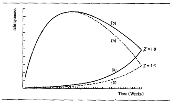
Figure 6.14 Theoretical biomass-time curves for age group 0 fish during one year when calculated from (a) simple exponential expressions for growth and mortality, and (b) “floodplain” expressions
Daget and Ecoutin (1976) also derived a model of biomass and production based on their growth equation for fish which have an annual growth arrest. Biomass is calculated from Bt=NtWt where:
Wt = 0.68 10-5 Lt³
Lt is derived from the formulae discussed in the section on growth and Nt is derived from the simple exponential mortality equation:
Wt = N0e-zt
The model was applied to Polypterus senegalus, giving good comparability with observed results. Estimates of production ranged from 528.5 kg/ha/yr (P/B=0.56) to 281.6 kg/ha/yr (P/B=1.12) for mortality coefficients z=0.04 and z=0.10 respectively. This illustrates the importance of correctly estimating mortality rate in deriving production and biomass values. The use of a constant mortality factor in this model is somewhat limiting and the abrupt termination of growth produces a rather sharply peaked annual biomass curve (Fig. 6.15) which does not appear to reflect the natural situation.
A more detailed simulation of the dynamics of a floodplain fish community was proposed by Welcome and Hagborg (1977) based on a combination of their growth and mortality models. By introducing density dependent mortality rates, and growth and recruitment which were dependent on the intensity of the simulated flood model enabled the exploration of the effects on a theoretical fish community of changes in high and low water components of the hyrdological regime. The simulation gave a series of curves for total ichthyomass derived from hydrological regimes in which either the flood intensity or the amount of water remaining in the system in the dry season could be varied independently of one another (Fig. 6.16). It indicated that differences in the flood regimes produce great differences in within the year ichthyomass whereas the magnitude of the population passing through to the following year largely depends on the amount of water remaining in the system at low water. They also indicated that the greater amount of water remaining in the system at low water the more the differences induced by the high water regime are transmitted to the following years. The curves in Fig. 6.16 were combined into a three dimensional plot of mean ichthyomass for different high and low water regimes (Fig. 6.17). Values for fish production per mean flooded area derived from this simulation agree well with the general findings on flood rivers ranging from 241 kg/ha/yr to 564 kg/ha/yr depending on flood regime with P/B values of between 1.35 and 1.77. Production and Biomass are both maximal in the higher floods but the ratio between them increases as the maximum area flooded decreases. This model, appropriately modified to the growth and mortality of local Oreochromis stocks has been applied to Lakes Alaotra and Ihotry in Madagascar (Moreau, 1980, 1982). Here the area under water in the dry season was 22 000 ha, whereas in the wet season the water flooded 57 000 ha. Apart from some differences in the numbers of fish the predictions of the model agreed closely with results obtained from experimental studies.
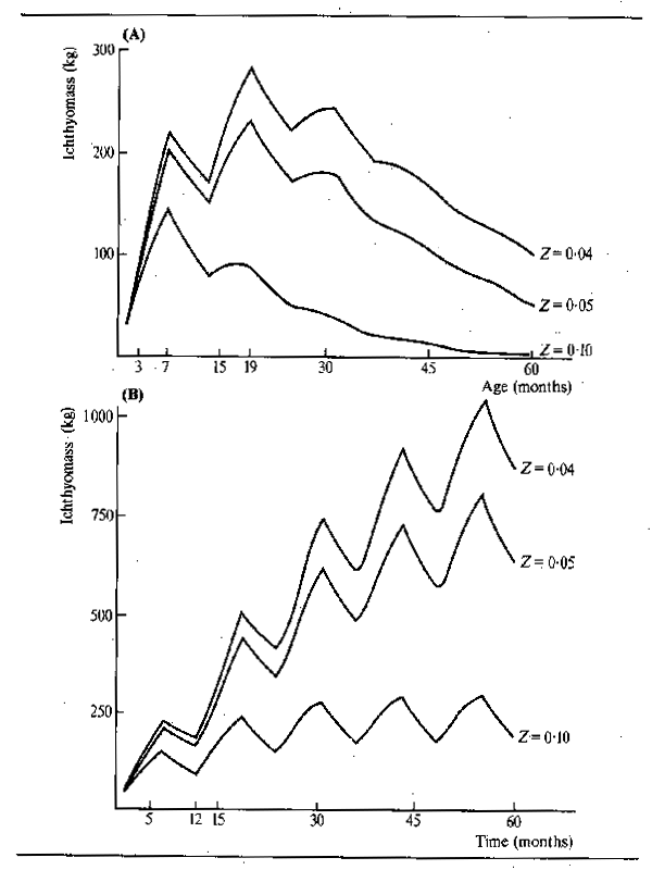
Figure 6.15 (A) Variations in ichthyomass of one cohort as a function of age for three different mortality coefficients; (B) Ichthyomass of population for three different mortality coefficients, assuming the same recruitment each year and the accumulation of cohorts. (After Daget and Ecoutin, 1976)
Figure 6.16 Computer generated curves showing changes in total ichthyomass with time for different flood regimes where (A) the low water regime is constant and the high water regime varies; and (B) the high water regime is constant and the low water regime varies. Also shown is a typical water regime (----). (After Welcomme and Hagborg, 1977)
These three models indicate a similar evolution of biomass throughout the year with a convex ichthyomass-time curve. According to this there is an initial rapid increase in ichthomass which attains a maximum at about bankfull on the declining flood and which would seem to represent the natural state fairly accurately. The models equally emphasise the great importance of the 0+ age group which contribute up to 80% of the total ichthyomass depending on the mortality rate. Both the shape of the biomass-time curve and the great preponderance of juvenile fish have important implications for the management of the fish community for fisheries. The variations in production and ichthyomass corresponding to differences in flood regimes predicted by the simulation suggest that equivalent yearto -year variations occur in the fish populations themselves. From records in many systems it is known that the catch does indeed fluctuate in this manner, and so presumably do production and ichthyomass.
Figure 6.17 Computer generated curves showing changes in population density (kg/ha) with time for different flood regimes where: (A) the low water regime is constant and the high water regime varies; and (B) the high water regime is constant and the low water regime varies. Also shown is a typical water regime (----). (After Welcomme and Hagborg, 1977)
Curves plotted from simulation for ichthyomass per unit area indicate that the population is very dispersed during the flood but concentrates rapidly as the water drains from the floodplain until bankfull (Fig. 6.17). This phase is followed by a steady attrition which reflects the real situation observed by Daget et al. (1973) in the Bandama and the University of Michigan et al. (1971) in the Kafue River. Changes in the ichthyomass per unit area are also evident from the seasonality of the fisheries which are at their most intense during those periods when the fish are concentrated in the late falling flood and the dry season.
![]()
![]()
![]()