Chapter 4
Estimation of soil loss

The Universal Soil Loss Equation (USLE) equates soil loss per unit area with the erosive power of rain, the amount arid velocity of runoff water, the erodibility of the soil, and mitigating factors due to vegetation cover, cultivation methods and soil conservation. It takes the form of an equation where all of these factors are multiplied together:

where:

The USLE equation has been modified-by separating the two elements of the cover and managment factor, C as follows:

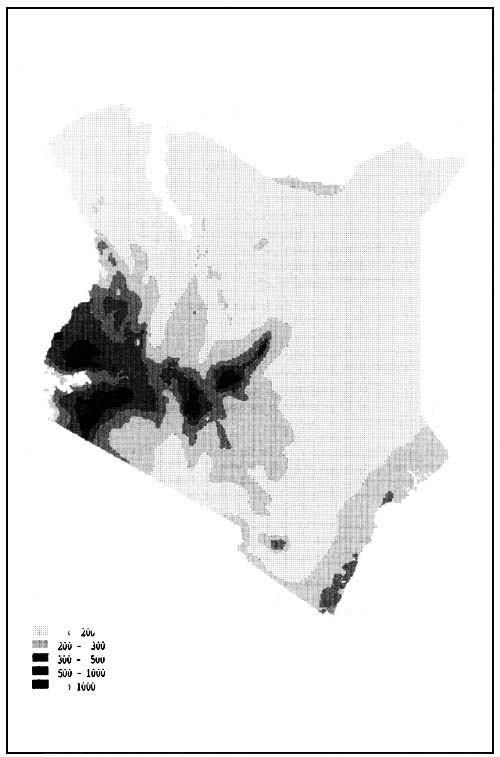
FIGURE 4.1
Generalized map of the rainfall erosivity factor (R)

Equation 4.2 is used in the model to estimate soil losses, which in turn are related to productivity losses and conservation needs. The procedure (Figure 2.1) consist of the following main steps:

1. Estimation of topsoil loss under specified vegetation/crop cover and management conditions for each land utilization type (LUT) as defined in the crop, livestock and fuelwood productivity models.

2. Estimation of productivity losses. The estimated soil losses are related to yield losses through a set of equations, taking into account the susceptibility of soils, and level of inputs.

3. Identification of conservation measures needed to reduce soil loss to an acceptable rate at quantified costs.

Each of the factors making up the soil loss equation 4.2 is quantified in turn, for a specified land use (LUT) or alternative land uses. Table 4.1 presents the attributes of land utilization types for crops. Attributes of land utilization types for pasture (livestock) and fuelwood are given in Technical Annexes 5 and 6 respectively.

4.1 Rainfall Erosivity (R)

4.1.1 Total erosivity of rain

Rainfall erosivity (R) is an aggregate measure of the amounts and intensities of individual rain storms over the year. It is related to total rainfall (Moore 1978; Hudson 1981; Wenner 1981).

An overall correlation of total rainfall with length of growing period (LGP) has been used for this model. Table 4.2 shows how R is related to LGP, and gives the equations relating both to mean annual rainfall.

Figure 4.1 presents a generalized map of the rainfall erosivity factor (R).

4.1.2 Seasonal erosivity of rain

The following criteria are used to define the seasonal distribution of erosive rain during the growing period.

TABLE 4.1
Attributes of land utilization types

Note. No production involving irrigation or other techniques using additional water. No flood control measures.

1. A ‘rainy season’ for the purpose of this model is defined as being 95% of the corresponding length of growing period (i.e. rainy season ending before the end of the growing period).

2. In years with one length of growing period (monomodal rainfall pattern) all the erosive rain is assumed to fall during the rainy season or the adjusted growing period.

3. In years with two lengths of growing period (bimodal rainfall pattern) and more, erosive rain in the rainy seasons is assumed to be proportional to the component lengths of growing periods.

4. It is assumed that 50 per cent of the erosive rain falls during the first quarter of a rainy season. The remainder of the erosive rains are distributed evenly through the rest of the season.

4.2 Soil Erodibility (K)

The estimate of soil erodibility is based on the nomograph produced for the Universal Soil Loss Equation (Wischmeier and Smith, 1978), with some modification to account for the behaviour of three groups of soils (Nitisols, Vertisols and Chernozems), which appear to be more erodible than the nomograph indicates. The range of estimated erodibility values for Kenya soils has been divided into 7 classes, as given at right.

Table 4.3 presents the soil erodibility class (K value) for each soil unit and for each soil texture listed as occurring in that unit. The mean K value of the soil erodibility class is used to calculate soil loss on any specified soil type. Figure 4.2 presents a generalized map of soil erodibility.

A cover of gravel or stones on the surface reduces erosion losses. The K value is reduced as follows to account for this protection:

1. Stony, gravelly or bouldery phases: stone cover is assumed to be 25%, K value is multiplied by 0.7.

2. Stone, gravel or boulder mantle phases: stone cover is assumed to be 50%, K value is multiplied by 0.4.

TABLE 4.2
Relationships between length of growing period (LGP), mean annual rainfall (MAR) and rainfall erosivity (R)

¹ LGP = 400 (1–1.0009 ^(170MAR))

² R = 117.6 (1.00105 ^(MAR))
(for MAR <2000 mm)
R = 0.5 (MAR) (for MAR >2000 mm)

FIGURE 4.2
Generalized map of the soil erodibility factor (K)

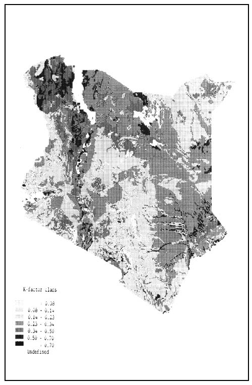
TABLE 4.3
Soil erodibilitv classification of soil units by soil texture

¹ Saline/sodic conditions reduce permeability of the subsoil, consequently the credibility factor K increases.

* Sodic/saline conditions are accounted for in these soils.

4.3 Slope-Length and Gradient (LS)

Two equations are used to give a figure combining the effects of the length and steepness of a slope; one for slopes up to 20% gradient, and one for steeper slopes (Arnoldus 1977). These are:

1. for slopes up to 20%

   LS = (L)0.5 × (0.0138 + 0.00965S + 0.00138S2)

   (4.3)

   where:  L = slope length (m)
   S = slope gradient (%)

TABLE 4.4
Associated slope classes

TABLE 4.5
Quartiles of slope classes

* 56% is taken to be the upper limit of slopes in the steepest slope class.

2. for slopes over 20%

Slope-gradients in Kenya are grouped into six classes by the Soil Survey of Kenya, and each mapping unit is assigned to one or a combination of up to three slope classes.

To each of the slope classes, associated slope classes have been assigned. These associated slope classes cover up to 10% of the land area. The inventoried slope classes and associated slope classes are presented in Table 4.4.

It is assumed for this model that a quarter of the land in each mapping unit is at the upper limit of the class to which it is assigned, a quarter is at the lower limit, and the two remaining quarters have intermediate slopes. Table 4.5 lists the slopes for each quarter of a mapping unit, for each slope class or combination of slope classes.

The length of the slope is assumed to be limited to 150 m on slopes up to 16% and 100 m on slopes more than 16%. These slope-lengths represent the average distance that runoff would cover before reaching a drainage channel. Figure 4.3 presents a generalized map of the slope factor (LS). Figure 4.4 presents a generalized map of potential erosion hazard. This map shows the combination of the erosivity factor (R), the erodibility factor (K) and the slope factor (LS).

4.4 Vegetation/Crop Cover (C*)

The total vegetation cover, and changes during the year, have to be related to the distribution of erosive rains to give an overall factor for protection by the vegetation canopy. In the case of annual crop production where different crops may be grown in rotation or alternated with fallows, an average protection factor is calculated for the full cycle.

Three types of land use are treated separately for estimating C*:

1. Pastures and bushland
2. Trees and shrubs (including forest and fuelwood plantations)
3. Annual crops (including 2-season crops)

4. Perennial crops.

4.4.1 Cover factors for pastures and bushland

The canopy cover of undisturbed vegetation, particularly the grass cover, is related to therainfall. Grass cover fluctuates over the year according to the rainfall pattern. The main factors altering the relationship are grazing and clearing for cultivation.

(a) Grass cover:

Table 4.6 shows the seasonal maximum and minimum cover of grass in relation to grazing pressure and lengths of growing period. The minimum cover is the condition found at the start of the growing period, while the maximum is assumed to be reached 60 days later. The increase in canopy cover between those dates is assumed to be linear.

The table is based on figures for average present-day grazing pressure, whereby cover is assumed to be 20% more dense when land is ungrazed, and 50% less dense when land is overgrazed.

The cover factor (C*) for grassland with a specified percentage cover is presented in Table 4.7.

(b) Establishment of grass and bush cover after cultivation:

Table 4.8 shows the time taken for grass and bush cover to reach the same density as natural pastures on uncultivated land, at different levels of inputs.

It is assumed that pastures are sown or planted at the high and intermediate levels of inputs but not at the low level of inputs.

FIGURE 4.3
Generalized map of the slope factor (LS)

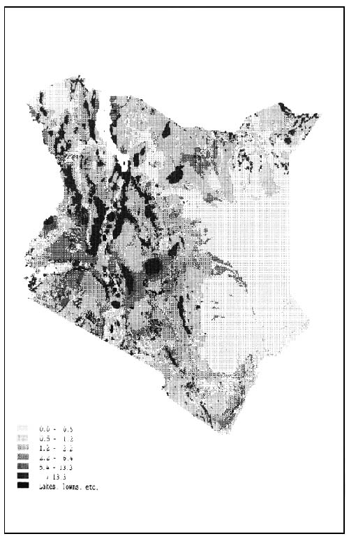
FIGURE 4.4
Generalized map of potential erosion hazard

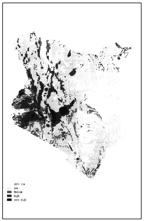
TABLE 4.6
Seasonal grass cover in relation to grazing by length of growing period (LGP)

Notes: (a) = Minimum cover at the end of the dry periods

(b) = Maximum cover at the end of the shorter LGP

(c) = Maximum cover at the end of the longer LGP

Source: Dunne, Aubrey and Wahome (1981).

TABLE 4.7
Cover factor (C*) for pasture

TABLE 4.8
Number of years required to reach full pasture cover by level of inputs circumstances

TABLE 4.9
Cover factor (C*) due to tree and shrub canopies of different heights (soil loss as proportion to loss from bare ground)

Source: Derived from Wischmeier and Smith (1978).

TABLE 4.10
Cover factor (C ) for undisturbed humid forest with litter layer at least 50 mm thick

Source: Adapted from Wischmeier and Smith (1978).

4.4.2 Cover factor for trees and shrubs

The canopy cover of trees and shrubs, natural or planted, is related to the rainfall, and once established the cover remains relatively constant. The main factors altering the relationship are browsing and cutting trees for fuel or other uses, and clearing for cultivation.

The protective effect of a tree canopy depends on its height above the ground; tall trees have little effect as drops from their branches are almost as erosive as the rain. Low shrubs are very effective. The amount of litter, on the ground is also very important; a deep layer of litter reduces erosion to almost nil.

Table 4.9 shows the cover factor for trees and shrubs of differing heights. To estimate the cover factor (C*) for woodland, the density of tree and shrub cover can be estimated from vegetation maps, while the appropriate seasonal grass cover is found from the length of growing period. The respective cover factors for trees and shrubs (Table 4.9) and for grass (Table 4.7) are then multiplied together.

The cover factor of humid forest is largely due to a thick layer of litter protecting the soil surface (Table 4.10). This factor is a single measure combining the effects of trees, undergrowth and litter.

TABLE 4.11
Crop growth stages as percentage of the total growth cycle, for annual crops

E -establishment

EV -early vegetative

LV - late vegetative

M - maturation

Source : Adapted from Doorenbos and Kassam (1979).

4.4.3 Cover factors for annual crops

The protective effect of an annual crop canopy varies from nil at planting to a maximum as the crop reaches maturity. The amount of erosion depends on the timing of the various stages of growth of a crop or combination of crops related to seasonal rainfall. The following steps are used to calculate the cover factor for an annual crop or crop mixture:

1. Set out the rainy seasons (in terms of length of growing period) on a calendar, with rainfall erosivity divided up into daily amounts according to the criteria in Section 4.1.2.

2. Set out the planting date, and the start and end of each stage of growth (crop stage) of each crop, on the calendar. Crop growth stages are given in Table 4.11, and they are:

   Establishment (E):	From sowing or planting to period establishment of 10% cover.
   Early vegetative (EV):	End of establishment to start of period bulking in root and tuber crops; end of establishment to start of stem elongation and yield formation in sugarcane; end of establishment to start of flowering in legumes, cotton and pineapple; end of establishment to start of head development in cereals and banana.
   Late vegetative (LV):	Bulking period in root and tuber period crops; yield formation period in sugarcane, legumes, cotton and pineapple; head development period and flowering in cereals and banana.
   Maturation (M):	Late yield formation and maturation period in root and tuber crops, sugarcane, legumes and cotton; yield formation and maturation in cereals and banana.

3. Find the maximum Leaf Area Index (LAI) of each crop. Leaf Area Index is used to estimate the percentage ground cover of the crop (Monteith 1969). Maximum LAI of single crops related to length of growing period and level of inputs are given in Table 4.12. When estimating maximum LAI for intercrops, it is suggested that the LAI of the first (main) crop is not reduced, but that of the second and subsequent crops is reduced by 25%.

4. Estimate crop cover at each crop stage of each crop.

   1. LAI at each crop stage is as follows:

      Crop Stage	LAI (percent of maximum)
      E - Establishment	5
      EV - Early vegetative		40
      LV - Late vegetative		100
      M - Maturation	80

   2. Crop cover is calculated from LAI by the equation:

      C = 100 (1-e (KL))

      (4.5)

      where:

      C = Crop ground cover %
      K = a constant based on geometry of crops: Table 4.13.
      L = LAI

TABLE 4.12
Maximum leaf area index (LAI) of individual crops by crop growth cycle

¹ LAI at low inputs level is half, and at intermediate inputs level is three quarters, of LAI at high inputs level.

Source: FAO (1978); Kassam (1980).

5. Estimate the cover of crop residues remaining after harvest. A relationship between crop residues and maximum LAI is given in Table 4.14.

6. For crop mixtures, record the crop cover for each crop stage on the calendar.

7. Estimate the combined crop cover of all crops in the mixture at each period on the calendar for which they are different using the equation:

   (4.6)

   where:

   Ti -the total percentage cover of i crops
   Ci -the percentage cover of the “ith” crop in the crop mixture.

TABLE 4.13
K values for leaf canopies of individual crops

Source: Derived from Monteith (1969).

TABLE 4.14
Amount of crop residues after harvest, in relation to maximum leaf area index of the crop

8. Estimate the cover factor for the combined annual crops for each period on the calendar Table 4.15.

9. Multiply the cover factor for each period by the daily rain erosivity and the number of days in each period. This gives the proportion of erosive rain that actually reaches the ground and is able to cause erosion. If the amounts for each period are totalled and divided by the annual erosivity R, the resultant fraction represents the annual cover factor C* for all the crops grown on the land.

TABLE 4.15
Cover factor (C*) for crops

source: Derived from Othieno (1972); Elwell and Stocking (1976); Barber and Thomas (1981), Colvin and Laflen (1981); Elwell and Stocking (1982).

The procedure described above can cover any combination of intercrops and sequential annual crops. To compute C*, the required variables for a given cropping system are:

-  Length of growing period (LGP)

-  LGP-Pattern (mono-modal, bimodal or trimodal)

-  Planting dates and length of growth cycle for each crop

-  Percentage of the growth cycle of each crop occupied by the different growth stages (Table 4.11)

TABLE 4.16
Possible maximum cover density of perennial crops, and number of years to reach it

TABLE 4.17
Soil loss ratios to bare fallow for flat cultivation, in relation to previous crop: subfactor M1

¹ Refer to Table 4.18.

² Crop stages refer to the dominant crop, in case of crop mixtures.

F - rough cultivation

E - sowing to establishment

EV - early vegetative

LV - late vegetative

M - maturation

R -residue or stubble

³ If land is cultivated after a bush or grass fallow, use this factor. The effect of fallow is given in Table 4.20.

-  Maximum LAI for each crop (Table 4.12)

-  Constant K for each crop, relating LAI to ground cover percent (Table 4.13)

-  Amount of crop residues, related to LAI (Table 4.14).

4.4.4 Reduction of crop cover due to soil factors and intermediate lengths of growing periods

Soil limitations and dry conditions reduce the growth of crops and hence the ground cover, to varying extents.

Soil factors may reduce productivity by reducing overall growth while the harvest index remains the same (for example soil fertility). In this case the leaf area index (LAI) would drop in proportion to the loss in yield, or they may reduce yield but not vegetative growth (for example nutrient imbalance, or shallow soils lacking moisture storage at the end of the rains), in which LAI may not be reduced significantly.

The soil factors used in the model represent a combination of both types of factors, so it is assumed for this model that the reduction of LAI due to soil limitations will be half the reduction in productivity. Thus if productivity is halved, LAI will be reduced by 25%.

Intermediate lengths of growing periods are growing periods in which rainfall does not exceed potential evapotranspiration (PET) at any time. The average rainfall is assumed to be 0.75 PET. This will create stress in vegetatively growing crops, and reduce the maximum cover. It is assumed that the reduction in cover would be as follows:

Crop stage E: No reduction (water requirement is below 0.75 PET at these stages)
Crop stages EV, LV and M: LAI is reduced by 25%.

4.4.5 Cover factors for perennial crops

Perennial crops are assumed to have a ‘constant’ cover once established. Tall perennial crops can be classified according to the height of the canopy, in the same way as trees and shrubs (Table 4.9). Low-growing bushy perennials (tea, pyrethrum) are classed as having the same protective effect as pasture (Table 4.15).

Possible rates of establishment and final maximum cover of perennial crops are presented in Table 4.16.

4.5 Management (M)

The management factor defines the effects of cultivation methods, mulches, manures and previous crops or pastures on soil erosion. Three subfactors are evaluated and multiplied together to estimate the management factor:

Management effects vary to some extent during the growing period, and the factors listed above are related to the crop stages of the dominant crop in the case of intercropped system. In a case where two successive crops are grown in a single continuous growing period, the second crop is regarded as a new seperate crop for estimating the duration of mulch effects.

TABLE4.18
Amount of crop residues remaining at the end of the dry period in relation to thermal regime, length of growing period and level of inputs

¹ a: < 1 t/ha c: 4–8 t/ha
b: 1–4 t/ha d: >8 t/ha
Residue values refer to land assessed as S1 (very suitable). Residue values are 25%, 50% and 75% lower respectively for land assessed as S2 (suitable) or S3 (moderately suitable) or S4 (marginally suitable).

Source: FAO(1978).

4.6 Physical Protection (P)

Physical soil conservation measures include both excavated works such as cut-off ditches or terraces and thus the use of vegetation in the form of trash lines or grass strips. They differ from cultural techniques in that they are applied at intervals on a slope, and they often involve taking a part of the land out of use for annual crops.

Physical conservation measures considered in the model are:

TABLE 4.19
Soil protection factors for cultivation techniques other than flat cultivation: subfactor M2

¹ see footnote in Table 4.17.

Small farms (manual or ox cultivation) - grass strips, trash lines, contour stone terraces, cut-off ditches (graded to outfall), converse terraces (‘fanya juu’, on the contour), step-terraces (for cash crops tea and coffee), and bench terraces (for cash crops tea and coffee).

Large farms (>50 ha, mechanically cultivated) - grass strips and narrow-based terraces (V-shaped terraces). These various measures act in different ways to reduce soil loss, and their effectiveness and costs are described in Section 6.

4.6.1 Systems designed to divert runoff water: channel terraces and bench terraces

Cut-off drains, narrow-based terraces and bench terraces divert runoff water across the slope, discharging it into channels away from the cultivated land. The effect is to reduce the length of slope between structures, and therefore soil erosion (Hammer 1981; Wenner 1981; Forster and Highfill 1983).

TABLE 4.20
Effect of previous grass or bush fallow, from farmyard manure, and surface mulches on soil loss ratios from cultivated land¹,²: subfactor M3

1 The figures assume a fallow of at least 3 years duration, for shorter fallows, multiply by 1.5 for two years fallow and 2.0 for 1 year fallow (If result > 1.0, use 1.0).

2 The values shown apply to cool conditions (thermal zones 6–8), for thermal zones 4–5 and 1–3 multiplication factors of 1.2 and 1.4 respectively to be applied (if result > 1.0, use 1.0).

3 Percent cover is the cover at the end of the dry season; the cover at the end of fallows shorter than 3 years is reduced by the amount shown in Table 4.8.

4 Farmyard manure is assumed to consist of cattle manure with little added straw or litter.

1. Cut-off drains: A cut-off drain is used to protect farmland from uncultivated slopes above. It is assumed to divert all runoff water, therefore slopes on farmland are defined as starting from the cut-off drain.

   The protective effect of a cut-off drain, in the absence of other conservation measure, is assumed in this model to reduce the slope length by half, i.e. to 75 m on slopes up to 16% and to 50 m on slopes over 16%.

2. Narrow based terraces: The maximum slope on which narrow-based terraces are recommended is 20%. Their protective effect is partly due to reduction in slope-length and partly due to silt deposition on the slope next to the terrace channel. Two P subfactors are used to calculate the protective effect: slope-length reduction factor (Table 4.21), and silt deposition factor (Table 4.22).

TABLE 4.21
Reduction of slope-length factor due to terracing, in relation to length of unprotected slopes

TABLE 4.22
P subfactor for deposition on narrow-base terraces in relation to terrace interval and channel gradient

3. Bench terraces and step terraces: Bench terraces are rarely constructed except on steep land intended for coffee planting. Step terraces (narrow terraces each with a single row of coffee) are recommended on slopes over 30%, and bench terraces on slopes between 12 and 30%. The effectiveness of terraces is due to both the reduction in slope-length depending on terrace interval and the reduction in slope-gradient on the terraces themselves.

   In the model, bench terraces are not considered at the low level of inputs. At the intermediate level of inputs, medium standard terraces without provision for water disposal are considered (P = 0.15). At the high level of inputs, high standard terraces with provision for water disposal are considered (P = 0.04).

TABLE 4.23
Protection subfactor (Ps)¹ for slope gradient reduction by converse terraces (based on an optimum vertical intrval of 1.5 m)

¹ The protection factor (Ps) is modified to account for soil permeability, and risk of damage by run-off and possible collapse of banks, by multiplying by: 3 × (K°.³²), where: K = soil erodibility.

TABLE 4.24
Protection subfactor (PI) for SIOPB length reduction by converse terraces

4.6.2 Systems designed for trapping silt and runoff: converse or ‘fanya juu’ terraces

Converse terraces are constructed by throwing soil upslope from a contour ditch. Runoff water and silt are trapped above the bank, which gradually builds up to form bench terraces. Their protective effect is due to reduction in both the length and gradient of slopes (Thomas, Barber and Moore 1980; Barber, Thomas and Moore 1981; Wenner 1981; Thomas 1983).

Three P subfactors are multiplied together to give a P factor for converse terraces:

-  Slope-gradient reduction factor (Table 4.23)

-  Slope-length reduction factor (Table 4.24)

-  Establishment of grass on terrace banks (Table 4.25)

4.6.3 Systems designed for trapping silt but no runoff: grass strips, trash lines and contour stone terraces

The purpose of these systems is to slow runoff, which increases infiltration next to the structure and causes some of the silt to be deposited (Mitchell 1965; Othieno 1965; Moore, Thomas and Barber 1979; Barber and Thomas 1981; Thomas 1983; Watson 1984). The result, as with converse terraces, is that a terrace is gradually built up, but the effective slope-length is only partly reduced on the amount of runoff absorbed.

1. Grass strips: The effect with grass strips is approximately equivalent to the slope-length reduction factor for converse terraces (Table 4.24). The effectiveness of grass strips depends on how well the grass is established, which in turn depends on length of growing period. The suggested modification to the slope-length reduction factor is the same as for converse terraces (Table 4.25).

2. Trash-lines: The effect with trash-lines is approximately equivalent to the slope-length reduction factor for converse terraces (Table 4.24). The effectiveness of trash-lines depends on the availability of materials. This is related to the net biomass production of the crop. A relation ship between the minimum possible spacing and the amount of crop residues is given in Table 4.26. The relationship between available residues, climate and level of inputs is given in Table 4.18 with the following adjust ments: a = 0 t/ha, b = 2 t/ha, c = 6 t/ha, d = 10 t/ha.

3. Contour stone terraces: The effect with trash-lines is approximately equivalent to the slope-length reduction factor for converse terraces (Table 4.24). The effectiveness of stone terraces depends on the availability of materials which in turn depends on the stoniness of the surface. Table 4.27 relates the percentage stone cover on the surface to the minimum possible terrace interval.

TABLE 4.25
Protection subfactor due to establishment of grass on terrace banks¹

¹Assuming good management. (Poor management, particularly uncontrolled grazing, would reduce the grass cover).

TABLE 4.26
Spacing of trash-lines related to availability of dry crop residues

TABLE 4.27
Possible intervals between stone terraces related to stone cover¹

¹ Stony phases are assumed to have a 10% cover of stones suitable for stone terraces, stone mantle phase 20% cover.