![]()
![]()
![]()
Sometimes the simplest way to estimate the effect of a physical process is to use an established equation, or formula, or charts and diagrams. The current trend is to call all such aids and solutions models, and they tend to become increasingly complicated and consequently dependent on computers to handle the mathematical processes.
As always, the objective must be clearly defined. Is information on the amount of erosion required because of concern about the loss of productivity or because a reservoir is silting up? Is the required end-product a number which will be used to design something or to give a better understanding of some part of the erosion process? Some discussions of the theory and practice of modelling are listed in the section on Further reading; this discussion will be limited to methods which can answer questions likely to arise in field projects.
The different kinds of models need a short explanation.
An empirical solution or model is one based on observation or experiment, and not derived from theory. It fits observed facts and allows the prediction of what will happen in certain circumstances, because what has happened before in those circumstances is known. The reliability of such methods depends on the database of experience: one might say "this will certainly happen" (because it always does), or "will probably happen" (because it usually does), or "it may happen" (because it sometimes does). An empirical solution may be a simple approximate relationship or a complex multiple regression equation.
Comparing the estimate obtained from one empirical method with that obtained from another empirical method without new experimental data is totally futile and unscientific, for example comparing the erosion index, EI30, with other empirical estimates of erosivity. The foundation and starting point of all empirical studies must be physical measurements.
A factor model is an empirical model where each of the variables is represented by a quantified factor, and then the factors are combined, for example by adding them up or by multiplying them. Examples are Cook's method for estimating runoff discussed in the section Maximum runoff rates, and the Universal Soil Loss Equation for estimating soil loss, discussed in the section Expirical models for estimating soil loss.
TABLE 11
Gathering time for small catchments (from Schwab et al. 1981)
| Average gradient in catchment (%) | 0.05 | 0.1 | 0.5 | 1.0 | 2.0 | 5.0 | 10.0 |
| Maximum length of flow (m) | Gathering time (min) |
||||||
| 100 200 500 1000 2000 3000 4000 5000 |
12 20 44 75 130 175 216 250 |
9 16 34 58 100 134 165 195 |
8 17 30 50 67 92 105 |
6 13 23 40 55 70 82 |
10 18 31 42 54 65 |
8 13 22 30 38 45 |
7 10 15 22 30 35 |
The term "black-box" model describes a model where the user feeds in defined items of information and takes out the answer without needing to know or understand what happens inside the black box. Such models are also called mystery models. These models can only be operated in the designed direction, that is all the inputs go into one side of the equation, and the answer is the output on the other side of the equation. A regrettably common misuse of one very important black box model, the Universal Soil Loss Equation, is to try to drive it in reverse and solve the equation for one of the inputs.
Empirical models are created from a database of experience obtained under certain conditions, so the model can be expected to work in those conditions. But it will not necessarily work under different conditions. No model can ever be truly universal - even process-based models need site-specific correction parameters. Ideally, each country or region should design its own prediction models to match its own conditions and to suit its database. Some examples are the Soil Loss Estimation Model for Southern Africa (SLEMSA), designed in Zimbabwe, and the European Soil Erosion Model (EUROSEM).
Procedures derived in the USA are built on a huge database from research, and there is a great temptation to apply them in less developed countries which cannot afford the time and expense to accumulate enough data to create local variations. A certain amount of extrapolation can be useful, for instance some components of the USLE may be borrowed, but this should be done with caution. The possibilities and the pitfalls of transferring USA technology on erosion prediction has been carefully studied (Foster, Moldenhauer and Wischmeier 1982).
A process-based model (also called an analytical component model) is able to mathematically explain each of the separate physical processes and then combine the separate effects. Because there are so many variables and so many mathematical computations, such models can only be operated through computers.
Stochastic models are useful particularly in hydrological studies and are based on the probabilities of the occurrence of events in a long time series. Both the last two types of model are outside the scope of the present discussion.
Finally, the accuracy and reliability of estimates from models can only be as good as the inputs. As the computer programmers put it, "garbage in, garbage out".
An estimate of the probable maximum rate of runoff may be required for the design of channels, drains or culverts, or to estimate maximum flood levels. Two simple empirical methods are described.
The rational formula is:
![]()
where:
Q is the rate of runoff in cubic metres per second,
I is the intensity in millimetres per hour,
A is the catchment area in hectares,
C is a dimensionless runoff coefficient.
The formula was derived originally in English units and owes part of its popularity to the fact that, when using the most convenient English units, C becomes dimensionless because of a fortunate numerical coincidence:
For rain falling at 1 in/hour on 1 acre, 43560 (acre to ft�)x 1/12 (inch/hour to ft/hour) x 1/3600 (hours to seconds) = 1.008 ft3/s, which for all practical purposes can be taken as unity, so in English units the formula is:
![]()
where:
Q is the rate of runoff in cubic feet per second,
I is the intensity in inches per hour,
A is the area in acres,
C is the same dimensionless factor as in the metric formula.
To solve the equation each of the three factors on the right-hand side needs to be known. The area A is measured by surveying, or from maps or aerial photographs.
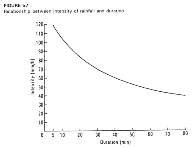
To get the value of intensity I it is first necessary to estimate the gathering time of the catchment, that is, the longest time taken by surface runoff to get from any point in the catchment to the outlet. Table 11 gives values of gathering time for catchments of various size and slopes. Next information on the highest intensity of rain which is likely to last for the given gathering time is needed. Local rainfall records should be used to estimate this if possible. When local records are not available an estimate can be made from Figure 57 which is derived from rainfall records in Australia and Africa. Short duration storms of less than five minutes can have extremely high intensities and this method should not be used for gathering times of five minutes or less. This figure shows the heaviest rainfall likely to occur on average once in 10 years. To get corresponding figures for shorter or longer periods the conversion factors of Table 12 can be used.
TABLE 12
Rainfall probability conversion factors for various return periods
| 2 years 5 years 10 years 25 years 50 years |
0.75 0.85 1.00 1.25 1.50 |
The coefficient C is a measure of the proportion of the rain which becomes runoff. On a corrugated-iron roof almost all of the rain would run off, so C would be almost 1.0, while a well-drained sandy soil, where nine-tenths of the rain soaks in, would have a C value of 0.1. Table 13 gives some values of C. Where the catchment has several different kinds of topography, or land use, a weighted average is found by combining the different values in proportion to the area of each.
TABLE 13
Values of runoff coefficient C (from Schwab et al. 1981)
| Topography and vegetation | Soil texture | ||
| Open sandy loam | Clay and silt loam | Tight clay | |
| Woodland Flat 0-5% slope Rolling 5-10% slope Hilly 10-30% slope |
0.10 0.25 0.30 |
0.30 0.35 0.50 |
0.40 0.50 0.60 |
| Pasture Flat Rolling Hilly |
0.10 0.16 0.22 |
0.30 0.36 0.42 |
0.40 0.55 0.60 |
| Cultivated Flat Rolling Hilly |
0.30 0.40 0.52 |
0.50 0.60 0.72 |
0.60 0.70 0.82 |
| Urban areas Flat Rolling |
30% of area impervious 0.40 0.50 |
50% of area impervious 0.55 0.65 |
70% of area impervious 0.65 0.80 |
This method was originally developed by an engineer of the US Soil Conservation Service, and requires an assessment of some of the main factors which affect runoff - the vegetative cover, the soil type and drainage, and the land slope. In Cook's original method there was a fourth factor of the extent of surface storage within the watershed, but trials have shown that the method can be simplified by ignoring this factor, without significant loss of its effectiveness.
For each of the three factors the catchment condition is compared with the conditions listed in Table 14. The description is found in the table which best fits the catchment, and the corresponding number is noted. Intermediate values can be used; for example, if half the catchment has heavy grass cover and the rest is not quite so dense, a value of 12 or 13 could be used. The arithmetic total of the number from each of the three columns is called the catchment characteristic (CC).
The area of the catchment is then measured, and using the area A and the catchment characteristic (CC), the maximum runoff can be read from Table 15. This gives the runoff for a 10-year probability, and the conversion factors given in Table 12 can be applied to get the corresponding figures for other time periods.
Another factor can be applied to take account of the shape of the catchment. Table 13 gives the runoff for a catchment which is roughly square or round. If the catchment is another shape the following conversion factors should be applied:
| Square or round catchment | Long and narrow catchment | Broad and short catchment |
| 1.0 | 0.8 | 1.25 |
TABLE 14
Values of Cook's watershed characteristics
| Cover | Soil type and drainage | Slope | |||
| Heavy grass | 10 | Deep, well-drained soils | 10 | Very flat to gentle | 5 |
| Scrub or medium grass | 15 | Deep, moderately pervious soil | 20 | Moderate | 10 |
| Cultivated lands | 20 | Soils of fair permeability and depth | 25 | Rolling | 15 |
| Bare or eroded | 25 | Shallow soils with impeded drainage | 30 | Hilly or steep | 20 |
| Medium heavy clays or rocky surfaces | 40 | Mountainous | 25 | ||
| Impervious surfacs and waterlogged soils | 50 | ||||
Select the most appropriate factor from each of these three lists and add them together.
Example: Heavy grass (10) on shallow soils with impeded drainage (30) and moderate slope (10):
CC = 10 + 30 + 10 = 50.
TABLE 15
Estimating runoff by Cook's method
CC from Table 14, A in hectares, runoff in m3/s
CC A |
25 | 30 | 35 | 40 | 45 | 50 | 55 | 60 | 65 | 70 | 75 | 80 |
| 5 10 15 20 30 40 50 75 100 150 200 250 300 350 400 450 500 |
0.2 0.3 0.5 0.6 0.8 1.1 1.2 1.6 1.8 2.1 2.8 3.5 4.2 4.9 5.6 6.3 7.0 |
0.3 0.5 0.8 1.0 1.3 1.5 1.8 2.4 3.2 4.1 5.5 6.5 7.0 8.4 10.0 10.5 11.0 |
0.4 0.7 1.1 1.4 1.8 2.1 2.5 3.6 4.7 6.3 8.4 9.7 10.5 12.6 14.4 15.5 17.0 |
0.5 0.9 1.4 1.8 2.3 2.8 3.5 4.9 6.4 8.8 11.7 13.2 14.7 17.2 19.4 21.5 23.5 |
0.7 1.1 1.7 2.2 2.9 3.5 4.6 6.3 8.3 11.6 15.3 17.2 19.6 23.2 25.6 28.5 31.0 |
0.9 1.4 2.0 2.7 3.6 4.5 5.8 8.0 10.4 14.7 19.1 21.7 25.2 30.2 33.6 36.5 40.5 |
1.1 1.7 2.4 3.2 4.4 5.5 7.1 9.9 12.7 18.2 23.3 27.0 31.5 37.8 42.2 45.5 51.0 |
1.3 2.0 2.9 3.8 5.3 6.6 8.5 11.9 15.4 21.8 28.0 32.9 38.5 46.3 51.0 55.5 62.0 |
1.5 2.4 3.4 4.4 6.3 7.8 10.0 14.0 18.2 25.6 33.1 39.6 46.2 53.8 60.0 65.5 73.0 |
1.7 2.8 4.0 5.1 7.3 9.1 11.6 16.4 21.2 29.9 38.5 46.9 54.6 62.5 69.3 76.0 84.0 |
1.9 3.2 4.6 5.8 8.4 10.5 13.3 18.9 24.5 35.0 45.0 55.0 63.7 71.5 79.5 86.5 95.0 |
2.1 3.7 5.2 6.5 9.5 12.3 15.1 21.7 28.0 40.6 52.5 63.7 73.5 81.0 90.0 97.5 106.5 |
In addition to knowing the probable rates of runoff, the total quantity which is likely to come from a watershed may be required. The total annual runoff is called the water yield, although one may be more interested in shorter periods, such as the monthly flow, or the amount from individudal storms. The usefulness of water for irrigation or domestic supplies not only depends upon the total amount, but also upon when it is available, and how reliable the supply will be. The average flow might be misleading if the likely variation on either side of the average, and the probable minimum flow are not known. The design of an irrigation scheme using a constant reliable flow would be very different from a scheme which requires storage to even out an unreliable and varying flow. Estimates of water availability therefore depend on having rainfall and streamflow records, and the longer and more reliable the records, the more accurate is the estimate based on them.
The methods of estimating water yield are quite different in arid climates and in humid climates. In humid climates the water table is fairly close to the surface most of the time, and higher than the bed of streams and rivers. There is therefore a steady seepage of groundwater into the streams, in addition to the direct runoff from storms. It is not possible to tell how much of the water in the stream has come from seepage flow and how much from storm flow, and so the total flow cannot be correlated with rainfall records; the only way to predict water yield is from past records of flow. In countries with sufficient data on streamflow, maps can be drawn showing isopleths, or lines of equal runoff. Naturally these resemble the rainfall maps, but the proportion of runoff is greater when the total rainfall is more, so the difference between low and high rainfall is magnified in runoff maps.
In arid regions there is no reservoir of groundwater, and so no seepage flow. The yield of runoff therefore consists entirely of storm runoff and this can be estimated from rainfall records.
The amount of runoff is the rainfall minus the losses, that is:
Q (runoff) = P (rainfall) - L (losses)
In semi-arid climates this method can be used to estimate annual runoff from annual rainfall by subtracting the estimated annual evapotranspiration. This is a function of land use and latitude, and can vary from 300 mm to 800 mm per year. If the cumulative runoff from a catchment is plotted against cumulative rainfall, the average losses can be determined from the slope of the graph as in Figure 58. Such a plot can be made using daily or weekly data or from individual storms.
In arid climates the loss is the infiltration and evaporation, and an estimate of yield can be obtained by applying the formula to each storm, assuming the same loss from each storm, with values from 10 mm to 20 mm per storm.
A more accurate method is to recognize that the losses are going to vary according to the amount of rainfall in the storm, and according to the amount of moisture which can be absorbed by the soil. This is the basis of the formula of the US Soil Conservation Service, which is:
![]()
where:
Q is the runoff in mm
I is the storm rainfall in mm
S is the amount of rainfall in mm which can soak into the soil during the storm.
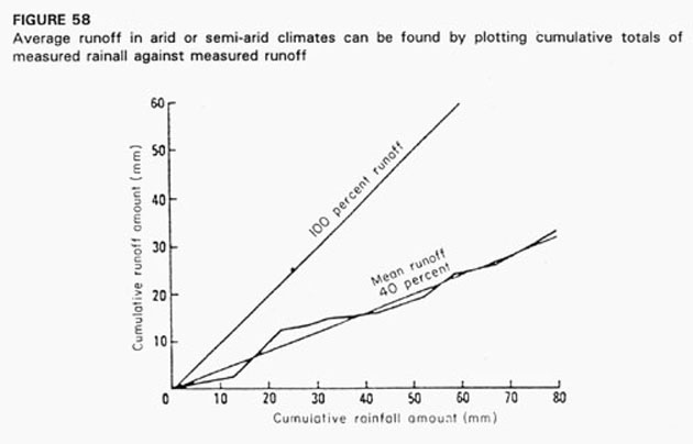
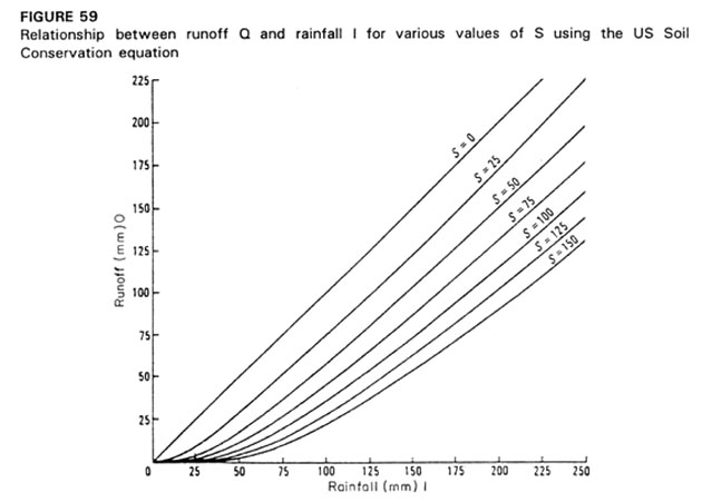
TABLE 16
Values of S (mm) for water yield formula. Intermediate values may be used (from USDA-SCS 1964)
| Soil type | Number of days since last storm which caused runoff | ||
| More than 5 | 2-5 | Less than 2 | |
| Good permeability, for example, deep sands | 150 | 75 | 50 |
| Medium permeability, for example, sandy clay loams and clay loams | 100 | 50 | 25 |
| Low permeability, for example, clays | 50 | 25 | 25 |
One possibility is to assume a constant value of S for a given catchment. More accurate estimates can be made by assuming that if storms occur in quick succession the soil will not have time to dry out in between. Table 16 shows some values of S which make allowance for this and for the different storage capacity of different soils. Figure 59 shows the above equation plotted for various values of S.
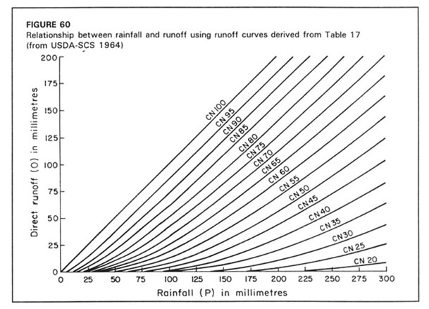
An alternative method of estimating the effect of conditions in the watershed, using some different variables, is known as the Soil Conservation Service Method of Runoff Curves. Four variables are considered and in each case a selection has to be made from a list of alternatives. Ten categories of land use or cover are offered, as shown in the first column of Table 17, with a choice of two or three appropriate soil conservation practices such as contouring (i.e. planting on the contour) and terracing (i.e. use of graded channel terraces). The hydrological condition of the catchment is graded good, fair or poor, and subjective assessments are called for in this category. For arable land, the hydrologic condition reflects whether the rotation will encourage infiltration and promote a good tilth. For grassland, it is assessed on the density of the vegetative cover, and more than 75% cover is 'good', while less than 50% is 'poor'. For forest lands, the criteria are the depth of litter and humus, and the compactness of the humus. Finally the soil is designated as one of four hydrologic soil groups described in Table 18.
A disadvantage of this method is that it relies on subjective (i.e. non-measurable) assessments as well as factual criteria. The variables are combined as in Table 17 to give the curve number which can range from 25 to 100. A weighted average can be calculated when conditions vary within the watershed. The procedure would be to first decide the area according to soil group, then according to land use, then obtain the curve number for each treatment and condition.
Figure 60 shows the runoff for curve numbers and rainfall amounts, and is clearly very similar in form to Figure 59, which is not surprising because the runoff curve number and S value are merely alternative estimators of the conditions in the watershed which will affect yield.
TABLE 17
Estimation of runoff curve numbers (from USDA-SCS 1964)
Land use or cover |
Treatment or practice | Hydrologic condition | Hydrologic soil group | |||
| A | B | C | D | |||
| Fallow | Straight row | - | 77 | 86 | 91 | 94 |
| Row crops | Straight row Straight row Contoured Contoured Terraced Terraced |
Poor Good Poor Good Poor Good |
72 67 70 65 66 62 |
81 78 79 75 74 71 |
88 85 84 82 80 78 |
91 89 88 86 82 81 |
| Small grain | Straight row Straight row Contoured Contoured Terraced Terraced |
Poor Good Poor Good Poor Good |
65 63 63 61 61 59 |
76 75 74 73 72 70 |
84 83 82 81 79 78 |
88 87 85 84 82 81 |
| Close seeded legumes or rotation meadow | Straight row Straight row Contoured Controued Terraced Teraced |
Poor Good Poor Good Poor Good |
66 58 64 55 63 51 |
77 72 75 69 73 67 |
85 81 83 78 80 76 |
89 85 85 83 83 80 |
| Pasture or range | Contoured Contoured Contoured |
Poor Fair Good Poor Fair Good |
68 49 39 47 25 6 |
79 69 61 67 59 35 |
86 79 74 81 75 70 |
89 84 80 88 83 79 |
| Meadow (permanent) | Good | 30 | 58 | 71 | 78 | |
| Woods (farm wood-lots) | Poor Fair Good |
45 36 25 |
66 60 55 |
77 73 70 |
83 79 77 |
|
| Farmsteads | - | 59 | 74 | 82 | 86 | |
| Roads | - | 74 | 84 | 90 | 92 | |
TABLE 18
Hydrologic soil groups (from USDA-SCS 1964)
| Hydrologic soil group | Runoff potential | Infiltration when wet | Typical soils |
| A | Low | High | Excessively drained sands and gravels |
| B | Moderate | Moderate | Medium textures |
| C | Medium | Slow | Fine texture or soils with a layer impeding downward drainage |
| D | High | Very slow | Swelling clays, claypan soils or shallow soils over impervious layers |
The runoff curve method may be applied to estimate runoff from an individual storm, or weekly, monthly, or annual rainfall. It is also possible to use it to derive estimates of maximum rates of runoff, and an example of this is reported in FAO (1976b) but the authors stress that this is an example of where extrapolation is only permissible to an area of similar climatic conditions where exact comparisons have been made, and should otherwise be treated with extreme caution.
Estimating soil loss is considerably more difficult than estimating runoff because there are so many variables, both occurring naturally such as soil and rainfall, and chosen management practices. As a result, models, whether empirical or process-based, are necessarily complex if they are to include the effect of all the variables.
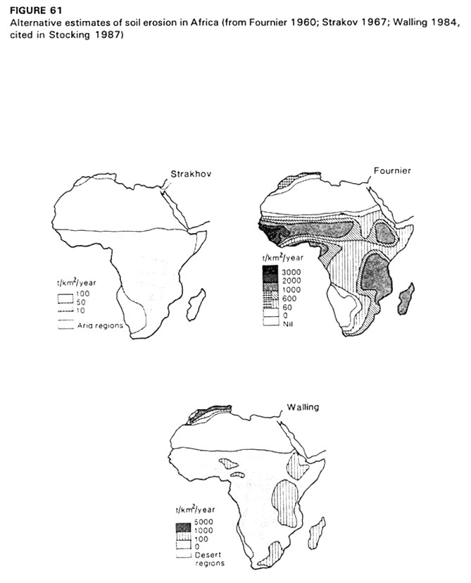
For some purposes, meaningful and useful estimates can be obtained from models, and the best example is the estimation of long-term average annual soil loss using by the Universal Soil Loss Equation (USLE). On the other hand, estimates of regional or national erosion are of very little significance or value, and the classic example of this is the three different estimates of suspended sediment yields within Africa compared by Stocking (1987) and shown in Figure 61.
Constructing a model based on physical processes is possible for small components of the erosion process; for example splash erosion involves only the energy of the rainfall, the extent to which the soil is covered and exposed by vegetation, and the soil type. Similarly, sediment transport requires only an understanding of the effects of particle size and velocity of flow. But a model of erosion in a field situation would require equations for both of these, and also equations to predict deposition and delivery ratio, none of which are presently available.
If the boundary conditions are limited, for example to soil loss from arable land of moderate slopes, it may be possible to set up an empirical black box model, and this has in fact been done successfully with the USLE. But there are other difficulties. The effect of extreme rainfall events may dominate the total amount of soil loss, particularly in the tropics and subtropics. In that case, the prediction of soil loss is heavily dependent upon rainfall probability studies.
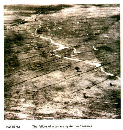
Another factor which can interfere with prediction equations is the effect of mechanical soil conservation systems overtopping, for example ridge and furrow systems, or failing from inadequate design or construction, as illustrated in Plate 43. Another aspect of erosion dominated by one-off events is mass movement from slips and landslides. The only way to deal with these three situations appears to be a combination of physical process modelling and stochastic modelling based on probability, both of which are outside the scope of this present discussion, except that it might perhaps be pointed out that the origin of 'stochastic' is the Greek for 'to guess'.
A basic difficulty with modelling soil loss is that the different forms of erosion have different causes and are influenced by different factors, so a model to predict erosion from arable land uses one group of parameters, but a model for gully erosion would use a very different set. In this discussion, estimating gully erosion is ignored because although the factors which cause gullies can be qualitatively identified, they cannot be quantified. Also estimates of watershed erosion are not included because deposition and delivery ratio cannot be quantified. However, the successful models for estimating soil loss from arable land, and some of the factors used in those models, are considered briefly.
The USLE has been a valuable and successful tool for nearly forty years. Its appeal has led to attempts to use it for purposes it was not designed for, and this has resulted in it sometimes being unjustly criticized. At one time this led the principal author of the system to explain how it should be and should not be used (Wischmeier 1976). The purpose is very simple and specific. It provides an estimate of the long-term average annual soil loss from segments of arable land under various cropping conditions. The application of this estimate is to enable farmers and soil conservation advisers to select combinations of land use, cropping practice, and soil conservation practices, which will keep the soil loss down to an acceptable level - in today's terms it would be said to ensure that the farming system is sustainable. Because it was designed for field use it had to be "easy to solve and include only factors whose value at a particular site can be determined from available data. Some potential details and refinements were sacrificed in the interests of utility" (Wischmeier 1976).
Some of the things the USLE is not intended to do (and should therefore not be criticized for not doing) are:
� Predicting sediment yield from a watershed, because it does not include deposition and delivery ratios
� Predicting soil loss from a single storm, because the factors are all long-term averages which smooth out the large variations
� Predicting soil loss outside the range of its own database without determining appropriate different values for the factors (for example the slope factor has only been experimentally determined up to 16%, and extrapolation beyond this should be tested by experimental studies)
� Separating the factors as if they were each independent. As Wischmeier (1976, p. 372) says "The relation of a particular parameter to soil loss is often appreciably influenced by the levels at which other parameters are present. To the extent that these interaction effects could be evaluated from existing data, they are reflected in the equation through the established procedures for computing local factor values. Factor R reflects the interaction of storm size and rain intensities". Wischmeier gives some other examples where interaction is partly accounted for, but the basic assumption is that each factor is an independent variable.
� Being used as a precise research tool to study the processes of erosion.
� Treating it as a mathematical equation which can be solved for one of the input factors, for example by measuring soil loss, estimating all the factors but K and then solving for K.
The equation is presented in the form
A = R x K x L x S x C x P
where:
A is the average annual soil loss in tonnes per hectare
R is a measure of the erosive forces of rainfall and runoff
K is the soil erodibility factor - a number which reflects the susceptibility of a soil type to erosion, i.e., it is the reciprocal of soil resistence to erosion
L is the length factor, a ratio which compares the soil loss with that from a field of specified length of 22.6 metres
S is the slope factor, a ratio which compares the soil loss with that from a field of specified slope of 9%
C is a crop management factor - a ratio which compares the soil loss with that from a field under a standard treatment of cultivated bare fallow.
P is the conservation practice factor - a ratio which compares the soil loss with that from a field with no conservation practice, i.e. ploughing up and down the slope.
The units require some explanation, particularly as they were originally derived in Imperial units, and the conversion into metric or SI units is the source of much error and confusion, compounded by the fact that the official USDA SCS reference on the subject (USDA 1978) contained errors which had to be corrected in a supplement of 1981.
The factors L, S, C and P are each dimensionless ratios which allow comparison of the site being estimated with the standard conditions of the database.
R, the erosivity factor, is computed by the erosion index (EI30) method which is the summation for each rainstorm of the kinetic energy (expressed in MJ/ha when using metric units in the USA or in J/m� in Europe), multiplied by the greatest amount of rain in any 30 minute period expressed in cm/h in USA or in mm/h in Europe.
K, the erodibility factor, is the average soil loss in tonnes per hectare for each unit of the metric R as calculated by the EI30 method. In effect, the units of K are arbitrarily chosen so that when multiplied by R in its unconventional units the product is in tonnes per hectare.
Although R and C are average annual factors, there is provision within the system for interaction between them. For example, a period in spring when the soil is newly ploughed and without any plant cover will be dangerous if the spring rains are highly erosive, but not a problem if the spring rains are gentle. Similarly, the effect on erosion of the state of the ground after harvest in the autumn will depend on whether or not the autumn rains are severe. To allow for this possibility, the growing season may be divided into periods and C and R values calculated for each period. The annual combined effect is the sum of the product for each period. Mathematically the effect is the same:
C x R = c1r1 + c2r2 + c3r3......
In the USA the wealth of data allows this calculation to be carried out with precision, and detailed charts and tables are provided in Agricultural Handbook 537 (USDA 1978). However, the crop rotations, cropping practices and rainfall distribution pattern are all specific to the USA, and in most other countries it will be more appropriate to use annual values of C and R.
The principle of separately quantifying the rainfall and soil erodibility factors in a format of multiplying them together is equally valid anywhere. There is, of course, no theoretical requirement for this format and one could construct a model in which the effects were combined by addition instead of multiplication, but this format is simple and it works. Similarly the concept of dimensionless ratios to compare a particular situation with a standard set of conditions is also transferable. It would be quite possible to leave out any of the present ratio factors or to insert others, but this would require a major research programme and the more practical approach is to try to establish local values of the existing factors.
It would be quite impractical to expect other countries to attempt to acquire a database comparable with that of the USA which used something like 10 000 plot years of experimental records to develop the USLE. It is therefore worth considering which of the principles and which of the USA-derived factors can be used in other countries.
The erosivity factor R is empirical, but the concept of basing it on rainfall energy and intensity has been confirmed in many countries. When attempts were first made to apply the USLE in the tropics, alarmingly high predictions of soil loss were discovered because the database of rainfall energy values obtained in the USA did not cover the high intensities of tropical rainfall, and extrapolation induced major errors. As a result, many attempts were made to find alternative empirical estimators of erosivity. However, later studies of high intensity rainfall in countries around the world established more realistic values for the energy of high intensity rainfall and these have now been incorporated into the USLE. In its present form calculation of erosivity values by the EI method are likely to be reasonable for most rainfall regimes.
The soil erodibility factor K is least likely to be transferable as several studies have shown that the USLE nomograph is not applicable to many tropical and sub-tropical soils (Vanelslande et al. 1984). The four factors fed into the nomograph are the percentage of silt plus very fine sand, the organic matter content, the soil structure, and the permeability. It is probable that the source of the discrepancy is that the silt and very fine sand content and the organic matter content are lower in tropical soils than in the medium-textured soils of mid-west USA. The only reliable way to establish local values for K is to use runoff plots under the standard conditions of bare fallow. It is commonly assumed that once the K value has been established for a soil this can be regarded as permanent. This is a useful simplification when the USLE is being used for its proper purpose, but in fact the value can change as a result of soil management; for example, the soil structure can change as a result of cultivation, and the organic matter content may be reduced by cropping or increased by manuring. There is also some evidence of seasonal variations in K values, particularly in climates with pronounced wet and dry seasons.
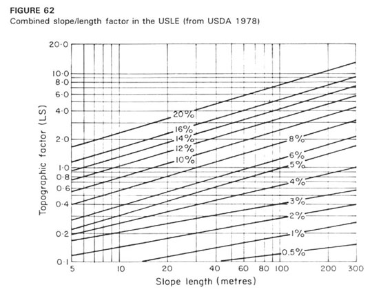
In the USLE the factors of slope length L and slope steepness S are combined together as shown in Figure 62, but this is only for convenience and the two factors derive from two separate and different relationships. The USA database for steepness factor S extends to 18? but it is quite likely that the physics of fluid flow and sediment transport will not be the same on very steep slopes, and this is a possible area for local investigation. The length factor L is less likely to vary, and the need to validate this relationship is of fairly low priority. The cover-management factor C certainly needs to be researched. The crop rotations and variations of the USA mid-West have been minutely researched and documented, and it is clear that the primary purpose of the C factor is to reflect how much protection is given to the soil by the vegetative cover. This principle will be the same under any cropping practice, but the tillage and cultivation practices may be quite different from those of the mid-West so local investigation of C is desirable.
The conservation practice P is rather crude in the USLE compared with the precision with which the other factors are calculated. One of the reasons is that the effect of major surface manipulation, such as graded channel terraces, cannot be satisfactorily evaluated with small plots as discussed in Chapter 3. Foster, Moldenhauer and Wischmeier (1982) suggest that most of the mechanical practices such as contouring, strip cropping, terraces, and contour furrows, which are used to support protection provided by crop rotation, canopy cover and residue mulches, are probably transferable. There are no values established in the USA for trash lines, grass strips, or agro-forestry practices, but these are the subject of research in several countries. Also there are no known values of P for bench terracing, but it can be argued that the mechanics of erosion on bench terraced land are so different that in its present form the USLE is not appropriate to this situation.
Since the introduction of USLE in 1958, there has been much research and many improvements, leading to the revised version of Agricultural Handbook 537 in 1978. Development has continued since then and a new version for operation on personal computers is at the stage of in-service field testing under the title Revised Universal Soil Loss Equation (RUSLE) (USDA 1991). A process-based model, Water Erosion Prediction Project (WEPP) is at a similar stage of development, and is expected to replace RUSLE at some time in the future. However, there will always be a place for USLE in its original function - to provide information to guide land use planning - because of its simplicity and ease of operation.
No other country has a database from experimental plots comparable with that of the USA which has the results from more than 10 000 plot years. Australia and Zimbabwe each have a significant base from long-running national research programmes with something of the order of 1000 plot years (for example 50 plots for 20 years). Many other countries have some runoff plots, and regional networks are stimulating many more, as described in Chapter 3. However, not all these experiments were designed to produce data for prediction equations and, as discussed in Chapter 3, the quality of the data often leaves much to be desired.
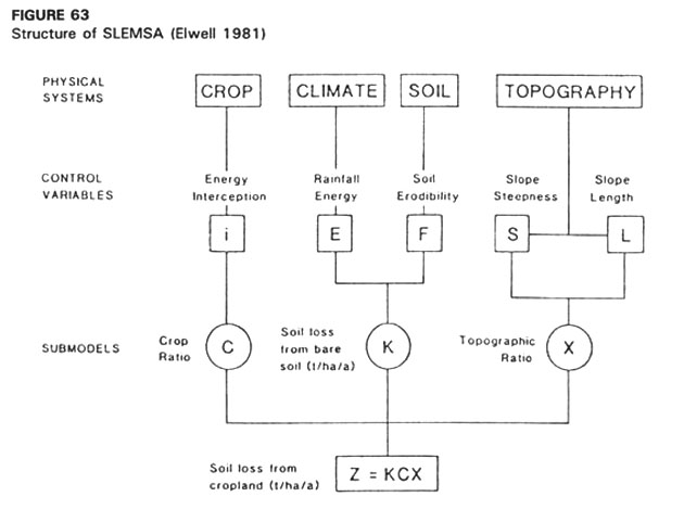
The question therefore, is how to make use of limited data in a system that allows progressive improvement as more data are acquired. A good example is the Soil Loss Estimation Model for Southern Africa (SLEMSA) (Elwell 1981; Elwell and Stocking 1982). The framework of the model in Figure 63 shows that it closely follows that of the USLE. The basic USLE equation in real units is A = RK, with modifying ratios C, L, S and P. The basic SLEMSA equation in real units is Z = K (a combination of rainfall E and erodibility F), with modifying ratios C derived from cover, and X from L and S. Both models estimate long-term average annual soil loss, and in both the combination of cover and rainfall energy can be done for each of smaller periods of time within the growing season.
The differences between the two models are that in SLEMSA:
� the P factor of USLE is left out because it is felt that the effect of local conservation practices can be allowed for in factors L or S within the topography system, or erodibility F in the soil system;
� the other factors are quantified by methods which are simpler to calculate or require less data;
R (in USLE) is replaced by E in SLEMSA, and is a measure of the total annual kinetic energy of the rainfall, which is easier to calculate from rainfall records than EI.
C in USLE is replaced by a different C in SLEMSA and is determined from i, the density of crop cover which is measured in the field at 10-day intervals over the 180-day growing season. C is expressed as a ratio of the soil lost from a cropped plot to that lost from a bare fallow. SLEMSA can be used to estimate the soil loss from rangeland using a slightly different sub-model to relate C to i.
K in USLE is replaced by F in SLEMSA which is a soil erodibility index and is based on soil type.
LS in USLE is replaced by X in SLEMSA calculated in a very similar manner but with slightly different equations.
In some cases it may be useful to be able to quantify relative changes in erosion, without trying to estimate absolute values of soil loss. A model is being developed in Indonesia, called INDEROSI, for this purpose (Gnagey 1991).
Empirical models all depend on a base of information collected on a few basic parameters, so a brief review of some of the methods of obtaining these data is appropriate.
The measurement of amount of rainfall is adequately described in all the meteorological manuals, and practical advice for field operation is in Pereira (1989). Rainfall intensity can be measured by specially designed instruments which continuously record the rate of rainfall, but the usual source of information is to compute it from charts from rainfall recorders as described in Hudson (1981b). Similarly, rainfall energy can be measured directly, through the medium of transducers or piezo-electric materials, or by acoustic devices which use a diaphragm to convert the energy into a sound signal which can be measured. The relationship between kinetic energy of rainfall and intensity has been studied in many countries around the world. The variations are shown in Figure 52, but there is doubt about how much these are real differences and how much due to different methods and techniques used in the measurements. It is clear that the general relationship is an increase of kinetic energy with intensity up to 75 mm/h, with little or no increase at higher intensities. A simple general equation is:
![]()
where:
E is the kinetic energy in J/m�/mm of rain
I intensity in mm/h
The capacity to cause rain splash is strongly correlated with kinetic energy. The direct measurement of absolute quantitative values is complicated, but relative values which will allow the comparison of the erosive power of different rainstorms or of different rainfall regimes can be measured effectively and simply in the field using a technique developed almost 50 years ago (Ellison 1944). The method is to expose to rainfall small metal containers filled with sand which are weighed in the oven-dry condition before and after exposure to the rain, as described in Lal (1988b).
Many methods have been derived for estimating the erodibility of soil from properties which can be measured in the laboratory, such as particle size and aggregate stability. Fourteen quantitative indexes are listed by Lal (1988b). For use in the Universal Soil Loss Equation, an empirical equation was derived using six components: percent silt plus very fine sand, percent organic matter, percent sand, soil structure and permeability, and this has been presented in the form of an easy-to-use nomograph (Wischmeier, Johnson and Cross 1971). The database for this was 13 bench-mark soils in the USA, mostly of medium texture, and of medium to poor structure. It has also been tested and found suitable for heavy-textured soils within the USA, but serious doubts have been expressed about its suitability for tropical soils in Hawaii, Tanzania and Nigeria by Vanelslande et al. (1984). Like erosivity, direct measurements in the field in absolute terms are difficult, but relative values for the comparison of different soil types can be carried out with a simple rainfall simulator.
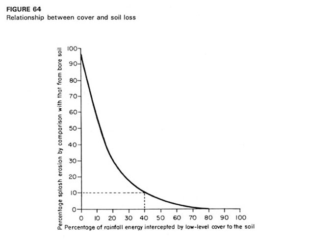
Erosion is greatly influenced by the extent to which the soil is protected from the energy of the rainfall or surface runoff by the vegetative cover. Many studies have shown that the relationship is non-linear, with a substantial reduction of erosion being caused by relatively small density of cover. The general relationship is shown in Figure 64. In SLEMSA, this relationship is used to create the index of the effectiveness of crop management. For the direct measurement of cover in the field, many methods have been suggested such as aerial photography, high altitude ground photography, stereoscopic photography and various methods to measure the light able to penetrate a crop canopy. The most successful method is that developed in Zimbabwe which has allowed the accumulation of a large database of measurements taken by extension workers. The instrument is a quadrat siting frame, similar to instruments used in botanic surveys, and uses an inclined mirror which by reflection allows the operator to look upwards through the canopy and assess the density. The method is explained by Stocking (1988).
![]()
![]()
![]()