![]()
![]()
![]()
The most difficult and crucial aspect in the estimation of change lies in the distinction between the variations pertaining to the object under study and those pertaining to the approach and instruments used or, in other words, between real changes and spurious changes. This problem acquires particular relevance where the changes to be detected are small and/or indistinct. With annual deforestation rates ranging between 0.5 and 1 percent, the changes in forest cover are relatively small and often poorly distinguishable even over a ten-year span.
When the objective of a survey is to achieve a detailed analysis of class-to-class transitions, it is essential that transition estimation be based on an approach that ensures the highest level of consistency, or coherence, between historical and recent observations, in order to reduce spurious change to a minimum.
During Phase I of the FRA 1990 Project a large number of forest inventories, repetitive surveys and monitoring studies was studied in detail to produce reliable and compatible pan-tropical forest statistics. This thorough review of existing information permitted a clear definition of the shortcomings of the approaches commonly used in the estimation of forest change.
Table (2.3) 1 below summarises the consistency between two (or more) periodic observations, using three traditional approaches and the approach adopted in the present survey.
| traditional monitoring approaches | present approach | |||
| Specific features of each temporal observation | Comparison of unrelated surveys | Comparison of repetitive surveys (same institution) | Single survey based on independent analysis of multi-date data | Single survey based on interdependent analysis of multi-date data |
| Classification | NO | YES | YES | YES |
| Remote sensing data, resolution, scale | NO | Y / N | YES | YES |
| Season of acquisition | NO | Y / N | Y / N | YES |
| Interpreter | NO | NO | Y / N | YES |
| Class delineation | NO | NO | NO | YES |
YES = consistency between historical and recent observations
NO = lack of consistency between historical and recent observations
Y / N = Not implicit in the approach; consistency between historical and recent observations varies case by case
The outcome of this review was that the most important element affecting the consistency of data sets, i.e., forest cover at date one and at date two, was how the data sources (satellite images, aerial photos) were related during the process of estimating the changes. The distinction between the characteristics and variations of land cover (object of study) and that of the satellite data used (instruments of the study) is best made when the two images are compared at every stage of the interpretation and subjected to a true/false judgement; assumptions based on one image are verified with the second image, weak evidence on one side could prove to be significant if confirmed on the other side. The information content of each satellite image, from being absolute, becomes relative.
In principle, this analysis could be carried out digitally as well as visually but in practice the digital approach is not yet able to cope with subtle variations in each image due, for example, to haze and shadows or seasonal variations in vegetation appearance. The advantages of being able to compare the two data sources and effect continuous relative adjustments made the visual approach the most suitable method of operational pan-tropical survey. Moreover, it was the most appropriate approach in terms of cost-effectiveness and timeliness.
However, an important question was: how can the subjectivity of class delineation be controlled?
Subjectivity is unavoidable in visual image interpretation. Such subjectivity in classification is particularly strong in classes with poorly contrasted boundaries. In fact, independent interpretations of two different images covering the same area will always present differences (or variability in class delineation) that do not represent real changes. This subjectivity alone, assuming that there is a high level of consistency among all other factors, might introduce sufficient “false changes” to make the monitoring results unreliable.
During the preparatory phase of the pan-tropical survey, with the purpose of identifying the most suitable visual interpretation procedure, three different approaches were tested on a selected site in Zaire and the results were compared. The results of this study, described in the Project Paper: “Interpretation of High Resolution Satellite Data and Compilation of Results for Forest Cover State and Changes Assessment; Test Site: Zaire” (R.Drigo, 1991) are summarised in Annex 6.
The outcome of this study was the design of an operational methodology for forest cover monitoring described in detail in the Field Document entitled “Procedure for Interpretation and Compilation of High Resolution Satellite Data for Assessment of Forest Cover State and Change”, Forest Resources Assessment 1990 Project (R. Drigo, 1991). The distinctive feature of the methodology is the interdependent interpretation procedure. Following this procedure, two images, acquired some ten years apart, are interpreted within a single interpretation process.
According to this approach, each class boundary is based on both images, thus eliminating any relative subjectivity in class delineation between the two images. Consequently, the changed areas are treated like other interpreted classes and have not been derived from the difference between two independent interpretations.
The interdependent interpretation procedure, shown in Figure (2.3) 1, can be summarised as follows:
The image showing better quality and interpretability, here called Image 1, is interpreted on a transparent overlay (Overlay 1), which is placed on top of the image.
The second image (Image 2) is then inserted between Image 1 and Overlay 1. A new overlay (Overlay 2) is placed and fixed on top of Overlay 1.
The interpretation of Image 2 is carried out on Overlay 2 with continuous reference to Overlay 1, as follows:
3.1 When the class boundary of Overlay 1 fits Image 2 it means that there are no changes and the same line is repeated over Overlay 2.
3.2 When the line of Overlay 1 does not fit Image 2 it means that there is a difference (not necessarily in land cover); the two images are therefore compared directly. Two outcomes are possible:
3.2.1 The line on Overlay 1 was wrong; there are no real changes in land cover. Overlay 1 is therefore corrected and the same line is drawn on Overlay 2.
3.2.2 There is a real change in land cover. A new class boundary is drawn on Overlay2 according to the features of Image 2.
The interpretation is carried out on both images with the production of two overlays, one for the recent image and one for the historical image. All lines correspond perfectly except where a class change has been detected.
| Figure (2.3) 1 : Interdependent Interpretation Procedure |
| Step 1 Interpretation of 1990 image on a trasparent film overlay (1990 overlay). The interpretation includes the delineation of Land Cover Classes (black lines) and control features (green lines). | 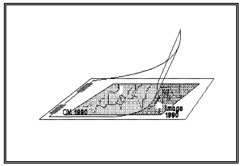 |
| Step 2 Insert 1980 image between 1990 image and 1990 overlay. Use the green control features to adjust the position of 1980 image to fit the 1990 overlay. | 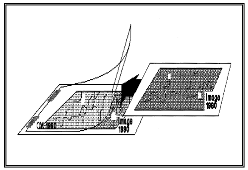 |
| Step 3 Interpret 1980 image (in blue on 1980 overlay) using the delineation on the 1990 overlay as a reference. Check and adjust constantly the position of the 1980 image with respect to the control features marked on 1990 overlay. | 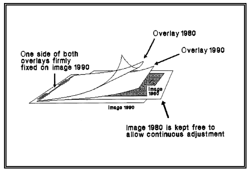 |
The result of the interpretation process will be:
The repetition of all unchanged class boundaries may seem redundant but it has been proved that only a thorough visual analysis permits the detection of all changes. Identifying and drawing the changes only through a visual scanning process tends to produce a systematic underestimation of changes, especially on images with highly fragmented patterns.
The continuous comparison of the two images increases the consistency and reliability not only of the changed but also of unchanged areas; often, while interpreting the second image, the need of modifying the interpretation of the first image arises, owing to new evidence. It can be concluded that, similar to the benefits of stereoscopy which increases the information content of two aerial photos taken from two different points in space, the combined “chronoscopic” use of two images taken at two points in time adds information to both images by showing the “behaviour” of both land cover and satellite imaging.
The effect of the interdependent interpretation procedure on the measurement error for both forest state and change estimates, as compared to the more conventional independent approach, is discussed in Section 4.4 “Evaluation of errors”.
An important effect of the interdependent interpretation procedure, in addition to the “thematic” co-registration of land cover classification, is the geometric co-registration of the resulting interpretation overlays.
In most cases, the historical and recent (analogue) images presented differing geometric corrections that produced, in spite of their common scale, considerable distortion between the images. In some cases this problem could have been avoided (cost and time constraints permitting) through digital co-registration of the satellite data but in many cases this solution was not practicable since the digital tapes of many historical images were unusable owing to obsolete data formats or to data loss (demagnetised tapes).
Relative geometric distortion is a problem that, if not properly solved, could seriously affect the validity of the resulting transition matrix1, which requires perfect spatial correspondence between the two interpretations. In the procedure of interpretation adopted, the recent image has been taken as geometric reference and the historical interpretation overlay has been designed to match it perfectly through continuous adjustment of the historical image to the recent overlay. This process was necessary in order to ensure that the image-to-image comparison was carried out on exactly the same area, in spite of any relative distortion.
The system of compilation and analysis at sampling unit level has been designed to produce two basic sets of statistics:
The following considerations ought to be kept in mind:
While the calculation of area is a relatively simple task that can be carried out in various ways through independent counts (by dot grid or planimeter), the compilation of the change matrix is possible only if there is a precise spatial relationship between the 1980 and 1990 data sets that allows the assessment of the same location on both dates. However, the need for a standard format and procedure to be used in developing country conditions made the use of a Geographic Information System (GIS) impractical in this phase of the survey.
The alternative solution was a system designed to run on standard Personal Computer (IBM compatible) using common spreadsheet software (LOTUS 123®), in combination with a dot grid of convenient size.
The system uses a dot grid on stable transparent film with 8 mm spacing where each dot, at the scale of 1:250,000, represents 400 hectares. The grid has a size of 100 × 100 dots (80 × 80 cm) in order to cover completely a full image at the scale 1:250,000. The dot spacing used represents a compromise between accuracy and convenience, the former increasing with the density of dots, and the latter resulting from practical aspects such as the time and difficulty of data recording.
Area measurement by dot grid is a systematic sampling procedure where each dot is the centre of a hypothetical square of given area. An error arises, however, because dots adjacent to a boundary do not represent the entire area of such a square. The percentage error tends to increase with the irregularity of the class boundary but diminishes with the number of dots counted. Since there is no bias introduced by the use of dot grid it is considered that this error, for aggregated results, is negligible (see Section 4.4 “Evaluation of errors” for further discussion).
The dot grid has column and row identification numbers that allow the unique identification of each dot which corresponds to a cell of a computerised spreadsheet file where the column and row identification numbers are also given.
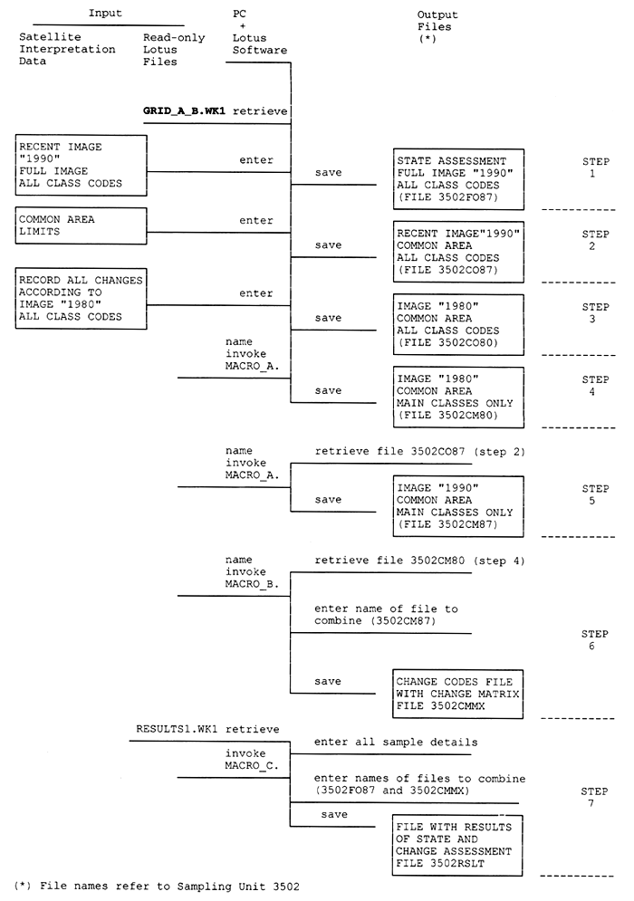
The Compilation System Flowchart, shown in Figure (2.4) 1, summarises the data entry and processing phases for one sampling unit. A detailed description of the compilation procedure, file coding system, files and programs used is given, as step-by-step instructions, in Field Document “Procedure for Interpretation and Compilation of High Resolution Satellite Data for Assessment of Forest Cover State and Change” (R. Drigo, 1991). This document, translated into three languages, has been used as the main reference manual in regional workshops and numerous training sessions.
When the data entry is completed for both the recent and historical images the two spreadsheet files created differ only for the classes which have changed during the intervening period between the images. From these two original files two new files are then created by collapsing all Additional Class codes to Main Class codes (codes from 0 to 9). These last two files are then processed to produce one “change file” showing one hundred unique codes that represent all possible combinations of the original ten classes. These unique change codes are created by multiplying all codes of the historical by one hundred and then by subtracting to them the value of the corresponding cell of the recent image. The result of this simple process is the “change file” which is then compiled in the form of a transition matrix, or change matrix, showing all class areas that remained unchanged (along the diagonal) and all the observed class-to-class transitions.
The outcome of the described compilation system, viz, the “result file”, includes, in addition to the two sets of data mentioned above i.e. state and change statistics, a detailed presentation of monitoring results based on the change matrix. These results describe the observed changes that occurred to the land cover categories according to the key to matrix interpretation presented under Section 2.2.1. By analysing the “result file” giving class areas, change matrix, deforestation and degradation rates, etc., the interpreter is able to verify their validity (or to carry out the necessary corrections) and to conclude the estimation process at sampling unit level.
An example of a standard “result file” is presented in Annex 11, for a particular location in North East India. A more thorough discussion of the same Sampling Unit is available in Section 4.1.
The spreadsheet files containing the class codes of both recent and historical images are subsequently used as input to produce simple raster maps with a 400-hectare pixel size, as discussed in Section 2.7 of the present report.
Figure (2.4) 1: Compilation System Flowchart
The results of the analysis of any individual sampling unit consist of (i) the areas of land cover classes at two separate times, defined by the dates of acquisition of the satellite images used; and (ii) the class-to-class changes observed for the interim period, in the form of a change matrix. In spite of giving priority to the acquisitions of 1980 and 1990, only a few suitable images were available from those particular years, the majority of them having been acquired some years earlier or later, as shown in the scattergram in Figure (2.5) 1.
| Figure (2.5) 1: Temporal distribution of recent and historical images of the 117 sampling units |
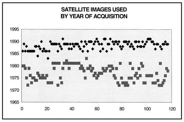
The varying years of acquisition of the Landsat scenes and varying intervening periods, prevented the direct inclusion of the original results into a homogeneous database for global and regional estimates. In order to be globally compatible, each set of results required a “temporal adjustment”, or standardisation, to the years 1980 and 1990.
If referring only to the variable forest cover 1980 and 1990, the adjustment is quite simple to carry out, by interpolating/extrapolating data on the basis of observed annual rates of change. This method of adjustment, however, cannot be applied to change matrices. At the same time it was considered of great importance that not only a few variables be standardised but the information content of the whole matrix, in order to allow aggregation and detailed analysis of change processes at regional and global levels.
This challenging task, as well as other analytical topics, has been the object of cooperative studies undertaken with the Swedish University of Agricultural Sciences (SUAS). The standardisation of the change matrices was finally accomplished through a mathematical method called “diagonalization” which is discussed in the Project paper “Estimates of Tropical Forest Cover, Deforestation and Matrices of Change” (E. Rovainen, PhD thesis, SUAS, 1994), summarised in Annex 7 and described briefly below.
The original n-year area matrix has been transformed into the n-year transition probability matrix; this has been done, row by row, by dividing the value of each cell by the “historical” total area of the class. The result is a transition matrix giving the probability that each historical class would remain stable or would change into any other class during the period observed.
The annual transition probability matrix is calculated from the n-year probability matrix through diagonalization.
Similarly, the 10-year transition probability matrix is calculated from the annual probability matrix.
The class areas in 1980 are estimated by applying the annual probability matrix 1980-t times to the classes of the historical image, where t=year of historical image.
The final 1980 – 1990 area transition matrix is then calculated by applying the 10-year probability matrix to the 1980 class areas.
Applied to all sampling units, the process of standardization produced a set of estimated change matrices covering comparable time periods and carrying the full information content of the original results.
The change matrices, original and standardized, represent a unique set of data on the land cover dynamics in the tropics. They represent the first consistent estimates of transition rates among nine relatively detailed tropical forest and other land cover classes between 1980 and 1990 that used compatible methods, compatible time periods and compatible definitions. Their value goes well beyond the scope of the present report and they represent only the first round of a continuous and evolving programme. The matrices can be aggregated or post-stratified under various viewpoints to provide revealing insight on the land cover change processes in the tropics.
For the present reporting purposes, it was considered necessary to aggregate and analyse the change matrices by ecological zone and by geographical region.
In addition to the three regions of Tropical Africa, Tropical Latin America and Tropical Asia, which represent the simple aggregation of the original sub-regions, the post-stratification was conducted on the basis of the following broad ecological zones, defined on the basis of rainfall:
Z1 - Wet and Very Moist (rainfall > 2000 mm)
Z2 - Moist (with short and long dry seasons) (rainfall of 1000–2000 mm)
Z3 - Sub-Dry to Very Dry (rainfall of 200–1000 mm)
Drier conditions with rainfall below 200 mm, such as Semi-arid and Arid zones, were implicitly excluded from the sampling universe in view of their lack of forest cover (see Section 2.1.1 “Sampling design”).
The main climatic characteristics of the ecological zones used are given in Annex 16, while their geographic distribution are shown in three regional maps in Section 4.2.3 “Ecological level results”.
The process of post-stratification was carried out according to classical statistical methods for sample survey that consider unequal probability of inclusion as follows:
The standardized change matrices were individually de-weighted according to the sampling fraction adopted in the original stratification.
The de-weighted matrices were aggregated according to the new stratification criteria.
The first and most important spatial output of the survey was the set of interpretation manuscripts resulting from the analysis of each sampling unit. These manuscripts, drawn on stable transparent film (hereafter called interpretation overlays), contain class codes and class delineation, and are the result of interdependent visual interpretation of historical and recent images. As a result of the interpretation approach both overlays, historical and recent, are co-registered to the scale and projection of the recent satellite image.
| Map specifications of the interpretation overlays | |
| Scale: | 1:250,000 |
| Projection: | Variable, usually Space Oblique Mercator (SOM), in all cases that of the recent “system corrected” Landsat image used in the sampling unit |
| Minimum mapping unit: | 3 × 3 mm for isolated classes 2 mm width for linear features |
In order to be used effectively in further spatial analysis, or simply for map production, these manuscripts must be converted into digital format and imported into a Geographical Information System (GIS). For the purpose of producing digital maps two different approaches have been followed:
Production of raster maps from spreadsheet files
Production of vector maps from original manuscripts (interpretation overlays)
These two options are quite different in terms of time, cost implications and outputs. The production of raster maps is simple and inexpensive but of lower spatial resolution while the production of vector maps is rather expensive and time consuming but maintains the full spatial resolution of the original manuscripts. From the point of view of thematic aspects such as classification and class-to-class transitions the two outputs are equivalent in maintaining full “thematic resolution”.
In view of the additional time and costs involved, the production of vector maps has only been initiated in selected areas along with the development of the most convenient vectorizing procedures. On the contrary the production of raster maps has been carried out systematically both for state and change maps and used during the phases of evaluation and validation of sampling units results.
Production of raster maps
As described in Section 2.4, for each SU a set of spreadsheet files was produced as result of the data entry by means of a dot grid. In addition to their use as input for the statistical analysis and further elaboration already described, these files were suitable to originate spatial information since the spatial relations among the 10,000 coded cells contained in each file truly represented the spatial features resulting from the interpretation of the satellite images. However, as a result of using a dot grid where each dot represents a square of 2 × 2 km, the map information is limited to a systematic sampling of the original class delineation with a ‘pixel size’ of 400 hectares.
This process of transformation from spreadsheet to raster map was effected by using the IDRISI® GIS package, which is simple and inexpensive, through the following steps:
State maps (historical and recent)
Change maps
The one hundred possible class transitions (including here also the “non-interpreted” class) have been consolidated, in a convenient color display, to 15 categories of change as shown in table (2.7) 1 below, following the principles discussed under Section 2.2.1 “Definition of forest and forest area changes”.
| Table (2.7) 1: Categories of change used in the legend of the raster change maps |
| Classes at date 2 | ||||||||||
| Classes at date 1 | closed forest | open forest | long fallow | fragmented forest | short fallow | shrubs | other land cover | water | plantations | Non-interpreted |
| closed forest | 7 | 4 | 4 | 2 | 1 | 1 | 1 | 1 | 6 | 14 |
| open forest | 11 | 7 | 4 | 2 | 1 | 1 | 1 | 1 | 6 | 14 |
| long fallow | 11 | 11 | 7 | 2 | 1 | 1 | 1 | 1 | 6 | 14 |
| fragmented forest | 12 | 12 | 12 | 8 | 3 | 3 | 3 | 3 | 10 | 14 |
| short fallow | 13 | 13 | 13 | 12 | 9 | 5 | 5 | 5 | 10 | 14 |
| shrubs | 13 | 13 | 13 | 12 | 10 | 9 | 5 | 5 | 10 | 14 |
| other land cover | 13 | 13 | 13 | 12 | 10 | 10 | 9 | 9 | 10 | 14 |
| water | 13 | 13 | 13 | 12 | 10 | 10 | 9 | 0 | 10 | 14 |
| plantations | 6 | 6 | 6 | 5 | 5 | 5 | 5 | 5 | 9 | 14 |
| non-interpreted | 14 | 14 | 14 | 14 | 14 | 14 | 14 | 14 | 14 | 14 |
| Code | Legend of Change Maps |
| 0 | Stable water |
| 1 | Deforestation |
| 2 | Fragmentation |
| 3 | Partial deforestation |
| 4 | Degradation |
| 5 | Decreased biomass |
| 6 | Forest <=> plantation |
| 7 | Stable forest |
| 8 | Stable fragmentation |
| 9 | Stable non-forest |
| 10 | Increased biomass |
| 11 | Forest amelioration |
| 12 | Partial afforestation |
| 13 | Natural afforestation |
| 14 | Non-visible |
An example raster maps of land cover state and change is presented in Section 4.1 as one of the products of individual sampling unit analysis.
Raster maps are being progressively transferred into the FRA 1990 Geographic Information System (GIS) in order to allow their integration with all other map layers of the project. The process of integration of the IDRISI raster maps into the GIS requires the completion of several transformations aimed at defining map coordinates and rotating them according to satellite orbit inclination. The main steps summarized below describe the automated standard approach followed in the absence of control points (G. Muammar, 1994):
new x = x·cos(α) y·sin(α) and new y = x·sin(α) + y·cos(α)
where α (angle of inclination of the image) = arcsin{sin(8.2)/cos(latitude)}
Other techniques of geo-referencing the raster maps have been tested for two sampling units (Peirsman, 1994). These techniques include (i) image to map, used as main reference for technique comparison; (ii) using corner point locations; and (iii) using a vector file location of corner points. The latter technique proved to be more accurate where accurate control point coordinates were available.
After checking the results of the transformation with reference GIS control features, the first grade approximation of the standard geo-referencing technique appeared to be acceptable in view of the coarse resolution of the raster maps. These maps are in fact more suitable for integrated statistical analysis and spatial models than for cartographic applications.
Production of vector maps
As stated above the statistical analysis and spatial representation of state and change of forests has been achieved, without loss of thematic resolution, by means of the raster maps. Nevertheless, spatial studies related to the analysis of “within-sample” processes might require a resolution higher than the one associated to the raster maps: i.e. landscape ecology studies dealing with spatial features, like shape, size, complexity of land cover features would produce more reliable output if based on the original 1:250,000 scale data.
In general terms, GIS applications oriented to “within-sample” studies would benefit from using high resolution data in a multi-layered analysis framework. In view of the above mentioned aspects, conversion of interpretation overlays has been initiated. A procedure was implemented to maximize the accuracy/cost ratio, involving the following steps:
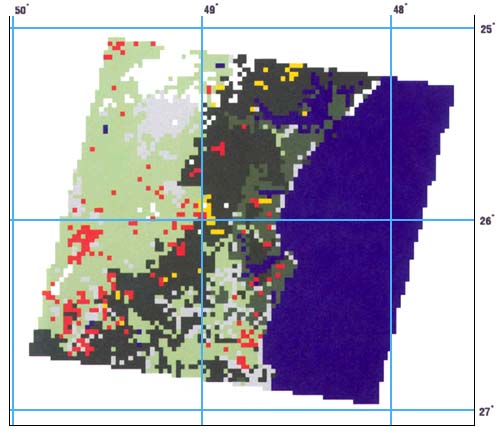
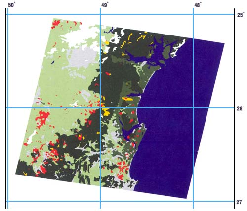
Figure (2.7) 1 shows the raster and vector maps derived from the same interpretation overlay of SU 3517, located in the south Brazilian State of Santa Catarina; this example shows the considerable gain in spatial resolution deriving from the vector approach. This approach is currently operational for the transformation of recent interpretation overlays into the FRA 1990 GIS databases. The conversion of historical interpretations is in a prototype phase in order to evaluate the most efficient way to store and retrieve changes as well as historical and recent data.
 |  |
 | OTHER LAND |  | SHRUBS |  | CLOSED FOREST |  | NON VISIBLE |
 | WATER |  | FRAGMENTED FOREST |  | SHORT FALLOW | ||
 | PLANTATIONS |  | OPEN FOREST |  | LONG FALLOW |
The estimation of the state and change of land cover classes is expressed as a bi-dimensional value such as area, area by class and area transition matrix. A transition of one million hectares from closed forest to other land cover is equal, in terms of area, to a transition of one million hectares from closed forest to open forest, except for an arbitrary conceptual categorization which tells us (if we so decide) that the first represents deforestation while the second represents degradation. One's way of perceiving this distinction remains subjective and descriptive, no matter how logical and documented, since the concept supporting it can be described but not measured.
Linking these conceptual elements (class, transition category) to a measurable parameter can serve the purpose of enriching the ambiguous level of conceptual subjectivity, expressed by the meaning we give to the various elements, with an element of quantitative comparability. A quantitative parameter such as biomass1 can provide this clarifying third dimension to the area results. The mean biomass value for a given class and the estimated biomass value gained or lost in class transition have absolute dimensions irrespective of how we categorize them.
The “biomass perspective” is a very interesting one in the analysis of land cover dynamics since it creates an unambiguous ranking system and it provides a quantitative estimation of the environmental impact of the changes such as the release or sequestration of woody biomass-related carbon.
The main problem consists in identifying reliable mean biomass density values to be allocated to each land cover class. In addition, the biomass value for a given class varies with specific site conditions.
Biomass data as such have been rarely measured in the field; most of the biomass information presently available derives from stand tables (the number of trees by diameter classes) and stemwood volumes which are typically measured and reported in forest inventories. Reliable methods have been developed for converting this available forest inventory information into biomass density estimates (Brown et al., 1989; Brown and Lugo, 1992; Gillespie et al., 1992; Brown and Iverson, 1992).
Volume-to-biomass conversion equations have been used in the FORIS database to estimate average country-level biomass densities for the main forest formations, viz, closed forest and open forest (sensu FORIS). Biomass density estimates have been related spatially and statistically to biophysical parameters, vegetation maps, population density data, etc., to produce forest biomass maps (Peninsular Malaysia, Brown et al., 1992; Continental South/Southeast Asia, Iverson et al., 1992; Africa region, Lorenzini, 1994).
The average biomass densities by main forest formation, produced in the studies above, have been correlated with ecological zoning and used to infer biomass values for the nine land cover classes for each zone. In some specific cases, such as the analysis of results of sampling unit 4409 located in north east India, discussed in Section 4.1, the class biomass values have been inferred from biomass estimates derived applying conversion equations to stand tables available from the exact study area. However, since no direct biomass measurement has so far been made in relation to the land cover classification here adopted, all estimates produced should be considered as indicative.
In the inference method followed to produce class biomass densities the available biomass values by main forest formation (from FORIS database and Biomass Maps) have been adjusted, on account of classification differences, to determine closed forest and open forest indicative values. In turn, values for long fallow and fragmented forest classes have been derived from the previous two classes on the basis of forest fraction and forest type of origin. The values for the remaining classes have been guesstimated as fractions of the relative closed forest value, used in this case as an indicator of productivity.
The main use for biomass values thus determined has been the positioning of the land cover classes along the Y axis of the woody biomass flux diagram developed in this study (see diagrams in sections 4.2.1, 4.2.2, 4.2.3). This diagram helps to visualize the biomass implications of class-to-class area transitions, to better understand the environmental toll of the various change processes and to compare them by ecological zone. A further contribution could be an indicative quantification of biomass loss and gain.
A more detailed quantification of biomass changes can be produced for the areas where sufficiently reliable biomass estimates are available. An example of such analysis is given in Annex 11 for one sampling unit located in North East India.
Table (2.8) 1 gives the inferred biomass values that have been used in the Woody Biomass Flux Diagrams shown in this report which describe the change processes at pan-tropical and ecological zone levels.
| Cover Classes | Ecological Zone | ALL ZONES | |||||
| Wet and Very Moist | Moist with Short and Long Dry Season | Sub-Dry to Very Dry | |||||
| (global mean) | |||||||
| Closed Forest | 300 | 200 | 120 | 225 | |||
| Open Forest | 100 | 80 | 60 | 90 | |||
| Long Fallow | 130 | 70 | 50 | 80 | |||
| Fragm. Forest (*) | 33 | 99 | 26.4 | 66 | 19.8 | 39.6 | 60 |
| Shrubs | 50 | 30 | 15 | 40 | |||
| Short Fallow | 40 | 20 | 10 | 30 | |||
| Other Land Cover | 10 | 5 | 3 | 7 | |||
| Water | 0 | 0 | 0 | 0 | |||
| Plantation | 150 | 100 | 100 | 110 | |||
Indicative estimates of the biomass “gradient” in each possible class transition (the difference between biomass in class of destination and class of origin) for the three ecological zones are given in Annex 8. This gradient, allocated to all possible class transitions, provides an interesting “third dimension” to class transitions or simple class relations that can be useful in the analysis of other issues, as discussed under section 4.4.3 “Evaluation of errors; classification errors”.
![]()
![]()
![]()