9. APPLICABILITY OF THE METHOD

As already mentioned the parameters a, g and S used to construct the limit curve are only a function of N and of the assumption that the population can or cannot be concave. Thus when the size of a target finite population is known, a random sample of size n will correspond to a predicted pessimistic accuracy computed by means of the function as defined in (7.5). Alternatively, if the population is of infinite size, predicted pessimistic accuracy values will be obtained through the use of the model described by (8.3).

The question arising here is whether the size of a finite population can be known to a reasonable degree of certainty. In most sample-based fishery surveys the population under study is finite and of known size as is, for instance, the case of total number of fishing craft operating from homeports. When the population size varies, then a maximum must be assumed.

The described model also provides information regarding critical sample size and breakpoints in the accuracy growth. As stated in Section 6.2 the critical sample size is when x=0.5 or sample size . It is clear that by simply computing a researcher can immediately determine at which sampling level the accuracy will start a steady increasing process towards 1. However, fixing a sample size by only considering the critical level does not always constitute an optimal approach for the following two reasons:

(a) For small populations the critical sample size and the predicted pessimistic accuracy at critical sample size will not necessarily indicate an expected accuracy of much higher level. This is particularly true in concave populations, such as the total set of recordings of fishing unit activities.

(b) Conversely, and particularly in large populations, an arbitrary selection of a very large sample size well beyond the critical point, may not prove a very cost-effective approach and the user may miss the opportunity of achieving about the same accuracy by using considerably smaller samples.

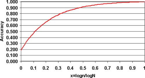
For these two reasons it is suggested that a table be constructed illustrating the predicted pessimistic accuracy for several sample sizes, so as to obtain more flexibility in the evaluation process of alternative sampling schemes. Table 9.1 and Figure 9.1 give an example of such a tabular approach using a simple electronic worksheet. The tabular data and the diagram refer to a concave population of size N=10 000. The worksheet was programmed to also include the intermediate computational steps and the resulting primary and secondary parameters used for the construction of the pessimistic accuracy curve A_(x).

The presented method also suggests that sampling criteria and practices should be reviewed and adjusted when the original target population is stratified into more homogeneous sub-populations. For instance, if a sample size is known to be effective when applied to a population before stratification, its effectiveness would be reduced if divided proportionally to the size of each of the stratified populations.

Table 9.1

PESSIMISTIC ACCURACY MODEL FOR FINITE POPULATIONS

INPUTTING PARAMETERS

Computed model parameters

Fig. 9.1 Pessimistic accuracy level