Gas monitoring and detection systems
Detection of gaseous concentrations is an essential prerequisite for both operational and safety reasons when any fumigation is attempted.
The requirements are the determination of excessive leaks from the fumigation enclosure (sheeted stack) or building, the concentrations achieved during the course of the fumigation, the concentration reduction during aeration, and protection of the fumigator from potential hazards associated with the fumigant. The threshold limit values (TLV's) have been revised with respect to the common grain fumigants in present use, which emphasizes the need for more accurate detection of environmental contaminants for operator safety.
Detection equipment must be used in preference to odour, even though some fumigants can be detected (not accurately;) this way. Phosphine possesses a garlic or carbide like odour (due to probably diphosphine, since pure phosphine is odourless) but may not be apparent due to preferential sorption on grain. Methyl bromide is odourless at low concentrations, and most formulations contain chloropicrin as a warning agent. Again, atmospheres containing methyl bromide may not be apparent to the fumigator due to different sorptive characteristics of chloropicrin (BP 112°C) as compared to methyl bromide (BP 3.6°C).
Detector Tubes
These are sealed glass tubes which, after the tips are removed, are inserted into a device and air is drawn through the tube. The fumigant then reacts chemically with the reagent coated granular filler and the color change is measured directly on the tube or with a calibration chart.
There are various types of pumps, such as Drager, Auer, Kitagawa and MSA.
Detector tubes are available for phosphine, methyl bromide, carbon tetrachloride, carbon disulfide, hydrocyanic peid, (acrylonitrile, ethylene oxide, carbon dioxide, ethylene dibromide, ethylene dichloride, oxygen, and other environmental contaminants.
1. Drager Multi Gas Detector
The pump consists of a simply designed, extremely strong bellows which requires practically no maintenance. The pump is easily operated by one hand and sucks in exactly 100 cm³ (100 ml) of gas per stroke, and measures the gas sample at the same time. The same bellows pump is used for the dust sampler to suck in the air sample for the analysis of dust concentrations.
The Drager tube is a glass tube fused at both ends and is chemically stable in this condition with a normal shelf life of approximately 2 years.
Operation
Both ends of the Drager tube are opened in the ampoule breaker eyelet by a "rotating, breaking motion", the eyelet being located next to the loop which retains the arrestor chain. The break off husk can also be used to open the ampoule. It prevents glass splinters from falling, and is provided in the carrying bag of the Gas Detector. The husk should be emptied from time to time.
The open tube is then inserted into the pump head so that the arrow of the tube points towards the pump and the writing surface towards the air inlet. The tube must be located firmly and tightly in the pump head so that no bypass air can be drawn into the pump.
During the test, the pump body is gripped by the working hand so that its base plate, which carries the pump head and takes the form of a recessed handle, is firmly located against the palm and the ball of the hand. The pump is held between the thumb and the base of the forefingers. The four fingers rest loosely on the front plate. The pump is operated by compressing the rubber bellows as far as the stop and releasing it.
When the pump is compressed, the air escapes form the bellows through the eyelet valve in the front panel and not through the tube, because this has a much higher flow resistance than the outlet valve. The suction of the pump begins with the opening of the four fingers which previously rested on the front panel. The fingers should be completely released from the panel, but the pump will still be firmly located between the thumb and the base of the forefingers. The compression springs within the bellows which are tensioned when the bellows are compressed, expand and the outlet valve is closed by the vacuum created in the bellows. The air then flows into the bellows, through the tube while the bellows expands to its original volume. The air volume drawn through the tube is determined by the dimensions and the stroke of the bellows. The end of the suction movement is reached when the arrestor chain is fully tensioned. The air velocity in the tube, which is decisive for the accuracy of measurements, is thus determined entirely by the spring force and the resistance of the Drager tube charge, which,is fixed during manufacture. The number of strokes prescribed for the various Drager tubes must be observed at each test (See Table 1).
2. Auer Gas-Detector(R), Auergesellschaft, GMBH, FRG
The Auer Gas-Detector(R) consists basically of a suction ball bulb and a pump body into which the detector tube is inserted. When the suction ball is compressed, a negative pressure is produced which draws the air to be sampled through the detector tube, the chemical composition of the indicating material being specifically developed for the gases and vapours being monitored showing a characteristic discolouration on their presence.
In most cases, a specific sample volume is drawn through the detector tube and the concentration of the substance to be detected is read from a scale according to the length of the stain or is evaluated by means of a table. Some detector tubes have only a very short discolouration (annular indication). In these cases, the sample volume needed to obtain the discolouration is equivalent to the concentration. Detector tubes have been developed for specific gases and vapours, or for broad spectrum application for a number of gases.
Table 1.
| GAS AND VAPOURS | DRAGER TUBE USED | ORDER CODE (1 pack) |
MEASUREMENT RANGE (20°C; 1013mbar): |
NO.OF STRODES | TLV (USA, 1979) |
| Perchloroethylene | Perchloroethylene 51a | 6.7 26699 | 5-50 ppm | 10 | 1000 ppm (5) |
| (Tetrachloroethylene) | " 10/b CH 30701 | 10-500 ppm | 3 | 100 ppm (5) | |
| " 0.1%1a 67 28021 | 0.1-1.4% vol. | 5 | - | ||
| 1,1,1-Trichloroethane | Trichloroethane 50/C | CH 21101 | 50-600 ppm | 10 | 350 ppm |
| (methyl chloroform) | |||||
| Phosphine | Phosphine 0.11a | CH 31101 0 | .1-4 ppm | 10 | 0.3 ppm |
| Phosphine 501a | CH 21201 | 50-1000 ppm | 3 | - | |
| 15-300 ppm | 10 | - | |||
| 150-3000 ppm | 1 | - | |||
| Phosphoric acid | Phosphoric acid | 67 2846 0.02 | ppm DDVP | 5 | 0.1 ppm |
| esters | esters 0.021a | DDVP |
The Auer Gas-Detector is simple with only 10 parts (locking screw; counting device, disc; washer; spring pin; spring; pump body; bushing; tube breaker; valve washer; and aspirator bulb for model 69), and can be taken apart and reassembled very quickly. The use of plastic and rubber makes the device largely resistant to corrosive gases and vapours; and combined with sturdy construction, virtually no maintenance is required. Where AUER Toximeter (TX), an electronically operated automatic pump for detector tubes is recommended.
OPERATING INSTRUCTION
Break off both tips of the detector tube in the tube breaker on the pump body of the Auer Gas Tester with a rotating movement.
Insert detector tube tightly into the pump body in the direction of the arrow printed on the tube (unless otherwise specified in the special instructions). Set disc counting device to the number given in the instructions for use of the detector tube used.
One hand operated, hold neck of suction ball between the tips of the index and middle fingers, apply thumb broadly to the operating ring at the bottom of the suction ball. Compress suction ball firmly in the direction of the pump body up to the stop. Do not try to squeeze out the residual air contained in the sides of the suction ball.
Take off thumb and allow suction ball to expand keeping the detector tube for another 5 seconds in the sampling area (unless otherwise specified). Repeat sampling procedure as often as indicated in the instructions for use of the detector tube. Move the disc counting device one by one digit before every stroke. The disc counting device is designed to engage at 0, which shows the user that the test is completed. Some detector tubes give off acid vapours during testing. Although the device is extremely resistant to these vapours, it is advisable to flush it after each use with a few blind strokes. Evaluate detector tube reading as described in the instructions for use.
Phosphine Detector Tubes
PH3-0.1: Used for detecting phosphine in air or technical gases over a range from 0.11Q0 ppm. For concentrations greater than 50 ppm and for checking TLV.
PH3-50: Used for detecting phosphine in a range from 50-2000 ppm.
The detector tubes have two scales, or calibrated for use with AUER Gas-Tester hand pump (G.T.), the other calibrated for use with the AUER Toximeter (TX).
Principle of Operation:
Reaction of phosphine with a silver compound and the formation of metallic silver. The indicator layer (white) is progressively discoloured zone for zone to brown in the aresence of phosphine.
The concentration indicated only applies for the selected location, and only for the moment in time the measurement was taken. Changes in concentration (evolution, gas leakage, formation of vapour clouds, etc) must be taken into consideration.
Accuracy:
Length of stain, more than 10 mm:t 10 to ± 15%
standard deviation
Length of stain, less than 10 mm:+ 15 to ± 25% standard
deviation
Measurement
| TUBE TYPE PUMP TYPE | : PH3-0.1 |
PH3-50 |
||
| :Gas tester (GT): | Toximeter (TX): | Gas Tester (GT): | Toximeter (TX) | |
| Connecting | Arrow points to- | Arrow pointing | Arrow in detector | Insert detector |
| detector tube | wards pump | away from pump | tube indicates | tube into rubber |
| flow direction | nozzle of pump. | |||
| (towards pump) | ||||
| Arrow indicates | ||||
| flow direction | ||||
| (away from pump) | ||||
| Range of | 10 strokes :0.1 | Switch position | 1 stroke (1 H) | Switch position |
| measurement | to 10 ppm | 10: 0.1-10 | 50 to 2000 ppm | 1: 50 to 2000 |
| Take reading on | ppm | For evaluation | ppm | |
| 10 stroke scale | Switch position | use GT scale | For evaluation | |
| (GT) | 1: 1 to 100 | use TX scale | ||
| 1 stroke: 1 to | ppm | |||
| 100 ppm | ||||
| Take reading on | ||||
| 10 stroke scale | ||||
| and multiply by | ||||
| 10. (GT) | ||||
| Suction time | 20 seconds per | Switch position | Approx. 25 sees. | Switch position |
| stroke includ- | 1: approx. 25 | per stroke | 1: approx 25 | |
| ing waiting time | seconds | seconds | ||
| Switch position | ||||
| 10: approx. 2.50 | ||||
| seconds | ||||
| GAS DETECTION EQUIPMENT | |
| Phosphine | Detector Tubes |
| Methyl bromide | Detector Tubes |
| Halide Gas Detector | |
| Thermal Conductivity Analyzer | |
| Interference Refractometer | |
| Carbon tetrachloride | Detector Tubes |
| Halide Detector | |
| Thermal Conductivity Analyzer | |
| Interference Refractometer | |
| Carbon disulfide | Detector Tubes |
| Thermal Conductivity Analyzer | |
| Hydrocyanic acid | Detector Tubes |
| Color Indicator | |
| Sulfuryl fluoride | Thermal Conductivity Analyzer |
Appendix
Fumigants can affect the commodity; or the nature of the commodity itself may affect the efficiency of a fumigant. Methyl bromide and phosphine may reduce seed viability, and methyl bromide can taint some products. Sorption of methyl bromide in oilseeds and other high oil content materials can reduce or even stop penetration of this gas into a bulk. A similar problem exists where hydrogen cyanide is used to fumigate high moisture content grains and other products.
Where economic advantage can be gained by marketing a product considered as residue free the choice of fumigant will be limited to carbon dioxide or phosphine. Carbon dioxide is the only fumigant that is acepted by the biodynamic and organic markets, as phosphine fumigation is considered to be a chemical treatment while application of carbon dioxide is not.
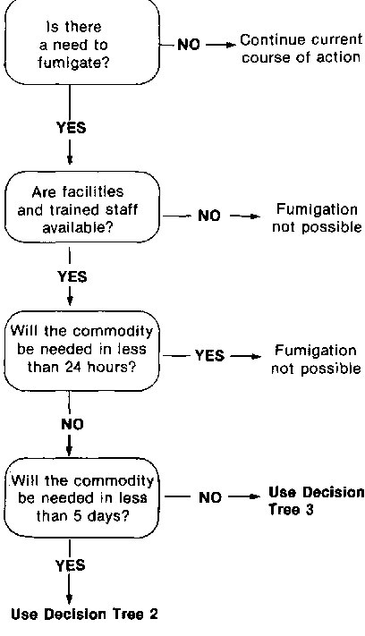
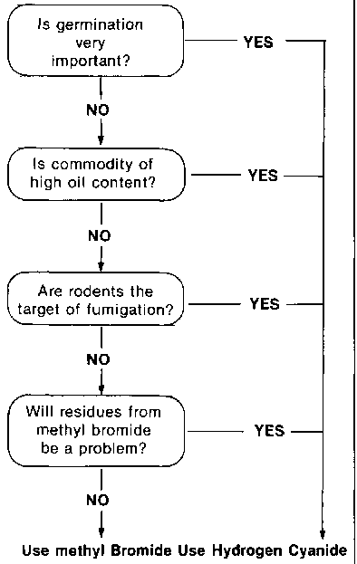
The following three 'decision-trees' provide a pathway that allows managers to make the choice of fumigant.
FUMIGATION DECISION TREE NO. 1
FUMIGATION DECISION TREE NO. 2
FUMIGATION DECISION TREE NO. 3
Is the fumication
enclosure close to occupied
dwellings that cannot be
vacated for the duration
of the treatment?
Is the fumigation
very close to a work
area in use?
Will the commodity
be needed in less
than 15 days,
Has carbon dioxide
an economic
advantage?
Use Phosphine
Use Carbon Dioxide
Are
Trogoderma spp.
present?
Will market accept
phosphine-treated
commodity?
Has phosphine
an economic
Use either Phosphine
or Carbon Dioxide
When and when not to use methyl bromide as a fumigant
Methyl bromide should be used:
Methyl bromide use should be avoided:.
When and where not to use hydrogen cyanide as a fumigant
Hydrogen cyanide is the fumigant of choice for
Hydrogen cyanide should not be used:
When and when not to use phosphine as a fumigant
Phosphine is the fumigant of choice:
Phosphine should not be used:
Dosage rates for hydrogen cyanide treatment of grain and empty stores.
| Situation | Dosage | Exposure Period |
| Empty warehouses, ships and barges, for control of residual insects | 8 g/m³ | 24 hours, with forced circulation |
| Empty warehouses, ships and barges for control of rodents | 2 g/m³ | 2 hours, with good distribution |
| Bulk grain with liquid HCN from cylinders, for insect control | 50 g/t | 24 hours, with recirculation |
| Bulk grain with calcium cyanide, as Ca(CN)2, for insect control | 80 g/t | 5 days |
| Bagged grain under gas-proof for insect sheets, for insect control | 50 g/t | 24 hours, with forced distribution |
Dosage parameters for methyl bromide applications to various commodities for control of insect pests.
| Commodity | S (g/m³ ) plus | M (g/tonne) | Exposure period (hours) |
| Paddy, brown and milled rice, barley | 10 | 0 | 24 |
| Wheat, oats, maize, pulses | 10 | 20 | 24 |
| Sorghum | 10 | 40 | 24 |
| Flour, nuts, oilseeds, rice bran* | 10 | 60 | 48 |
| Oilseed cakes and meals* | 10 | 120 | 48 |
*These commodities should not be fumigated with methyl bromide unless required by contractual obligations or for quarantine reasons. Other fumigants are to be preferred.
When and when not to use carbon dioxide as a fumigant
Carbon dioxide is the fumigant of choice:
Carbon dioxide should not be used:
The aim with a carbon dioxide fumigation is to expose any insects present to a concentration of carbon dioxide above 35% for longer than 15 days. The dosage applied to achieve this will depend on:
As these factors will vary vastly between enclosures, a set dosage per tonne of commodity can be only a rough guide to the required dosage. A more economic and reliable approach is to observe the concentration within the enclosure and to stop adding gas when the average concentration (or the concentration at the top of the enclosure) reaches 75° carbon dioxide. In a correctly sealed enclosure, this will give a concentration of greater than 34% at 15 days after treatment.
In a sealed enclosure meeting the pressure test standard, a concentration of greater than 75% carbon dioxide should require no more than 1.7 kg of carbon dioxide per cubic metre of total storage space. The amount less than 1.7 kg/m3 will depend on the actual values attributed to 1-5 above. In a full storage with effectively zero headspace, the dose rate to achieve greater than 75% has been observed to be about 1.2 kg of carbon dioxide per tonne.
Dosage rates for phosphine
| Temperature (°C) | Dosage rate (g/m³) | Equivalent commodity dosage* (g/tonne) | Minimum exposure period (days) Admixture & recirculation | Surface application |
| Above 25 | 1.5 | 2 | 7 | 20 |
| 15-25 | 1.5 | 2 | 10 | 20 |
* Rate appropriate for raw, whole cereal grains. Commodity dosage rates should be used only when structures are full or have little no head remaining.
Calculation of Ct products
Effective fumigation with methyl bromide can ensured only if the recommended Ct product has been reached or exceeded. The Ct product is calculated by multiplying the concentration of fumigant observed in grams per cubic metre (g/m³ ) by the time in hours (h) that the concentration has been present, and is recorded in gram hours per cubic metre (9 h/m³). If the gas concentration within the enclosure were to remain constant, the Ct product could be estimated simply by multiplying the concentration by exposure time. However, in any real fumigation the gas concentration always changes with time. The Ct product then has to be calculated by adding together the component Ct products obtained from the average concentration of sequential observations and multiplying by the time interval between them. The best approximation of true total Ct product is obtained with a large number of concentration observations it an exposure. However, practical constraints often limit the number of observations that can be made. Concentrations should be measured at about 2, 4, 12, and 24 hours after dosing. If a 48-hour exposure is used, readings at about 36 and 48 hours should also be taken. A Ct product cannot be calculated on fewer than two concentration measurements. If only two readings are possible the first must be taken after gas mixing is complete and the second must indicate a quantifiable concentration (that is, more than zero or a trace).
In fumigations under gas-proof sheeting where gas loss rates are very high, the Ct product is best calculated by using the geometric mean. This is done by multiplying together two observed gas concentrations (as grams per cubic metre), taken one after the other then multiplying the square root of this number by the time interval (in hours) between the two readings. This can be expressed as the equation:
![]()
where
Tn is the time the reading was taken
in hours
Tn+1 is the time the second reading was taken in hours
Cn is the concentration reading at Tn in
g/m³
Cn+1 is the concentration reading at Tn+1
in g/m³
Ctn,n+1 is the calculated Ct product between Tn
and Tn+1 in g h/m³
The Ct products obtained from a series of readings may then be added to calculate the cumulative Ct product for the whole exposure period (see examples 1 and 2 in this Appendix). It is this value that is used to indicate the success or failure of a fumigation. The calculation is easily carried out on a simple electronic calculator with a square root function.
In well sealed enclosures that have passed a pressure where gas loss rates are low, the Ct product may be calculated by using the arithmetic mean. This is done by adding together two observed gas concentrations (as grams per cubic metre), taken one after the other, and multiplying half of this number by the time interval (in hours) between the two readings. This can be expressed as the equation:
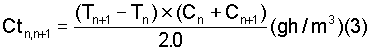
where:
Tn is the time the first reading was
taken in hours
Tn+1 is the time the second reading was taken in hours
Cn is the concentration reading at Tn in g/m³
Cn+1 in g/m³
Ctn,n+1 is the calculated Ct product between Tn
and Tn+1, in g h/m³
The Ct products obtained from a series of readings may then be added to calculate the cumulative Ct product for the fumigation (see example 3). It is this value that is used to indicate the success or failure of a fumigation.
It is possible to add gas during the course of an exposure to maintain a minimum gas concentration and so achieve a prescribed or statutory Ct product.
Note: whichever method of calculating the Ct product is used, it is important the gas within the enclosure is well mixed and the concentrations have become approximately even by the time the first concentration reading used in the calculation (e.g. 2 hours in a bag stack) have been taken. Pairs of observations containing a zero or unquantifiably low (e.g. trace) concentration cannot be used to obtain a valid contribution towards a cumulative Ct product.
Worked examples of Ct calculation
The following examples (based on hypothetical methyl bromide fumigations) are given to illustrate the steps needed to calculate Ct products using either equation 1 or 2 above.
Example I
A fumigation under gas-proof sheets with a high loss rate, where the Ct product is calculated on the basis of equation 1. This is the type of result that would be expected in many commercial fumigations or where the commodity is very sorbtive.
Example of calculation
Using equation 1 for the period form 2 to 4 hours
Ct2,4 = (4.0-2.0) × (20.0 x 15.5)1/2 = 2.0 × (310.0)1/2 = 2.0 × 17.6 = 35.2
That is, the Ct for the period between the obserations = the time between the observation x the square root of the product of the concentrations at the two observation times.
Readings:
| Time (hours) |
Time step (hours) | Concentration (g/m³) | Ct product (g h/m³) | Cumulative Ct (g h/m³) | Comments |
| 0.0 | - | - | - | - | End of gassing |
| 2.0 | 2.0 | 20.0 | + | 0.0 | Ct cannot be calculated |
| 4.0 | 2.0 | 15.5 | 35.2 | 35.0 | |
| 12.0 | 8.0 | 6.2 | 78.4 | 113.6 | |
| 24.0 | 12.0 | 2.0 | 42.3 | 155.9 | |
| 36.0 | 12.0 | trace | * | 155.9 | Ct cannot be calculated |
| 48.0 | 12.0 | 0.0 | * | 155.9 | Ct cannot be calculated |
+ No contribution to Ct as most probably not mixed by this
time and sample may not be representative of concentrations as a
whole.
*Ct for this time period cannot be calculated as final value is
less than a quantifiable concentration.
Example 2
A fumigation with a very high loss rate where top up gas is added to ensure that the required Ct product is achieved. Here the Ct product is calculated using equation 1. This is the type of result that can be expected from a poorly sealed fumigation under under-sheets, or a fumigation of a very sorbtive commodity where a contractual or quarantine target dose (either Ct or minimum concentration over a set time) has been specified.
Readings:
| Time (hours) | Time step (hours) | Concentration (g/m³) | Ct product (g h/m³) | Cumulative Ct (g h/m³) | Comments |
| 0.0 | - | - | - | - | End of gassing |
| 2.0 | 2.0 | 20.00 | + | 0.0 | Ct cannot be calculated |
| 4.0 | 2.0 | 15.5 | 35.2 | 35.2 | |
| 7.0 | 3.0 | 10.0 | 37.3 | 72.5 | Top up started |
| 8.0 | 1.0 | 19.5 | 14.0 | 86.5 | Top up finished |
| 15.0 | 7.0 | 10.0 | 97.7 | 184.2 | Top up started |
| 16.0 | 1.0 | 15.5 | 12.4 | 196.6 | Top up finished |
| 24.0 | 8.0 | 4.0 | 63.0 | 259.6 | |
| 36.0 | 12.0 | trace | * | 259.6 | Ct cannot be calculated |
| 48.0 | 12.0 | 0.0 | * | 259.6 | Ct cannot be calculated |
+ No contribution to Ct as gas most probably not mixed by this time and sample may not be representative of concentrations as a whole.
*Ct for this time period connot be calculated as final value is less than a quantifiable concentration.
Example 3
A fumigation in a well sealed enclosure that has passed the pressure test and where the gas loss rate is low. Here the Ct product is calculated using equation 2. This type of fumigation is only likely to occur in an extremely well sealed enclosure with a relatively nonsorbtive comodity.
Readings:
| Time (hours) | Time step (hours) | Concentration (g/m³) | Ct product (g h/m³) | Cumulative Ct (g h/m³) | Comments |
| 0.0 | - | - | - | - | End of gassing |
| 2.0 | 2.0 | 19.8 | + | 0.0 | Ct cannot be calculated |
| 4.0 | 2.0 | 19.7 | 39.5 | 39.5 | |
| 12.0 | 8.0 | 19.0 | 154.8 | 194.3 | |
| 24.02.0 | 18.1 | 222.6 | 416.9 | ||
| 36.0 | 12.0 | 17.2 | 211.8 | 628.6 | |
| 48.0 | 12.0 | 16.4 | 201.6 | 830.2 |
+ No contribution to Ct as gas most probably not mixed by this time and sample may not be representative of concentrations as a whole.
Example equation 2 for the period from 2 to 4 hours
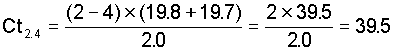
That is the Ct for the period between the observations = the time between between the observation × the sum of the concentrations at the two observation times - 2.0