![]()
![]()
![]()
Techniques for analysis of adaptation have been developed for three main objectives:
definition of adaptation strategies for breeding programmes;
variety recommendation; and
identification of optimal test or selection locations.
Different objectives may co-exist in the analysis of one data set, but partially different approaches may be required. Differences between the first and second objectives concerning the relevant GL interaction effects and the underlying criteria for subregion definition are outlined in Chapter 2 and summarized in Table 5.1. Different procedures are required for subregion definition within each analytical technique; consequently, results for site classification generally differ between the two objectives. In particular, location classification based on the similarity between relevant GL effects is essential for the preliminary definition of distinct subregions for breeding. On the other hand, accurate modelling of best-yielding material across locations is required for the definition of subregions for genotype recommendation. Data transformation to compensate for heterogeneity of genotypic variance among sites is useful for definition of adaptation strategies (see Section 5.6). The indications for this objective in terms of relevant GL effects and data transformation are also useful for identifying optimal test or selection locations (see Section 6.2), although subregion definition may not be implied in this case.
TABLE 5.1 - Major differences between two possible objectives for analysis of adaptation
|
Item |
Adaptation strategy for breeding |
Genotype |
|
Relevant GL effects |
All a |
Crossover between best-ranking entries |
|
Subregion definition |
Site similarity for GL effects b |
Best-ranking genotype(s) |
|
Possible data transformation c |
Useful |
Useless |
a Related to lack of genetic correlation among locations.
b Complemented by comparison of wide vs. specific adaptation.
c Against heterogeneity of genotypic variance among sites.
Scope for modelling
Modelling GL interaction effects through joint linear regression, AMMI (additive main effects and multiplicative interaction) factorial regression etc. is justified, as a simplified description of genotype responses helps target genotypes and understand adaptation patterns. Modelling is also important for improving the prediction of future responses of genotypes in comparison with observed data, because the portion of uncontrolled error variation in the GL interaction (so-called "noise") tends to be removed from the meaningful "pattern" portion retained in the model (Gauch, 1990, 1992). The higher predictive ability of expected (i.e. modelled) yields relative to observed yields for genotype-location combinations can be justified by the fact that model parameters (hence, all plot values used for estimation of these parameters), rather than only plot values for the specific genotype by location cell mean, concur to the estimation. In fact, genotype ranks on individual sites based on observed data can be quite different from those expected according to the selected AMMI model (Crossa et al., 1990; Gauch and Zobel, 1997; Ebdon and Gauch, 2002). Differences often concern also the best-yielding genotypes on the sites; these "winning" genotypes become a smaller subset based on expected data (thereby facilitating cultivar recommendation), because noise effects allowing lower-yielding material to occasionally win have been removed (Gauch and Zobel, 1997). For trials repeated in time, the noise portion relates mainly to the error term for GL interaction, i.e. non-repeatable GL interaction or GY interaction within locations. On the basis of results from an independent data set (Annicchiarico et al., unpublished results), when recommendation of the two top-yielding cultivars in each location was based on yield response modelled by factorial regression, joint regression or AMMI analysis (as reported in the case study in Section 8.3), yield gains were on average 4 to 5 percent higher than when recommendation was based on observed yields for each site. The elimination of noise effects from genotype responses - of crucial importance for making variety recommendation - may also be contemplated when grouping sites on the basis of their similarity for these responses in the context of subregion definition for breeding.
Analytical approaches
The following techniques - namely, joint regression model, AMMI models, factorial regression models including environmental covariates and pattern analysis - are a subset of those which may be adopted for analysis of adaptation. Major techniques not described here include:
shifted multiplicative model (Cornelius et al., 1992; Crossa et al., 1993, 1995);
application of canonical variates analysis (Seif et al., 1979; Calinski et al., 1987);
factorial regression model contemplating genotypic as well as environmental covariates (Denis, 1988; van Eeuwijk et al., 1996);
reduced rank factorial regression (van Eeuwijk, 1992, 1995);
partial least squares regression (Aastveit and Martens, 1986; Talbot and Wheelwright, 1989; Vargas et al., 1998); and
a recent method based on a Bayesian approach for variety recommendation (Theobald et al., 2002).
Ordinary crop simulation models offer sometimes excellent potential (e.g. Hammer and Vanderlip, 1989), but their adoption is generally limited by the difficulty of reliably representing the GL effects by empirically-estimated genetic coefficients - also in view of the large amount of experimental data required (Hunt et al., 1993; Russell et al., 1993). Recent models incorporating gene action may be considered an integration rather than an alternative to current models for analysis of adaptation, mainly for assessing the value of single traits and combinations of traits in the context of a given adaptation target (Hoogenboom et al., 1997; Chapman et al., 2002). However, some models may also support decisions on adaptation strategies, by simulating results of multi-environment trials and even the outcome of different selection strategies (Cooper et al., 1999).
Joint linear regression analysis was developed by Yates and Cochran (1938). Slightly different models have since been proposed by Finlay and Wilkinson (1963), Eberhart and Russell (1966), Perkins and Jinks (1968) and others (as reviewed by DeLacy et al., 1996a). According to Perkins and Jinks' model (applied to GL rather than GE interaction analysis), the GLij effects (relative to the genotype i and the location j) are modelled as a function of the location main effect (Lj) or the location mean value (mj), which represents an indicator of the ecological potential of the site for the crop (positive Lj or high mj = high potential; negative Lj or low mj = low potential):
GLij = βi Lj + dij = αi + βi mj + dij
where βi is the regression coefficient of the genotype i and dij is the deviation from the model, i.e. the residual GL interaction; in the second expression an intercept value αi (equal to -m βi, where m = grand mean) is also present. The β coefficients, with a mean value equal to zero, and the genotype mean yields are the relevant estimated parameters of genotype adaptation, since the genotype merit on a given site depends on its mean yield and the expected GL interaction effect (which varies according to the β coefficient). Largely positive and negative β values, if associated with relatively high mean yield, result in specific adaptation to high-yielding (favourable) and low-yielding (unfavourable) sites, respectively. Conversely, β values around zero indicate a lack of specific adaptation (and wide adaptation, if combined with high mean yield). No definite indication on genotype adaptive responses can be inferred solely from β values: for example, an entry that is highly susceptible to a disease occurring on high-yielding sites would show a negative β value even if it was only mid-ranking for yield on low-yielding sites.
Estimation and test of model parameters
In the joint regression analysis table, the GL interaction SS (relative to ANOVA models in Tables 4.1 through 4.3) is partitioned into two components relating, respectively, to:
heterogeneity of genotype regressions; and
deviations from regressions.
The SS proportion accounted for by heterogeneity (model R2) may be obtained by summing up the model SS across separate regression analyses of GL effects performed for each individual genotype, and calculating the proportion in the total SS in the regressions. The complement to one of this value indicates the proportion of GL variation accounted for by deviations from regressions. As an alternative, SS values for genotype regressions and deviations from regressions can be provided by model and error SS, respectively, in the analysis of covariance of all GL effects as a function of genotype main effect and genotype × site mean yield interaction (which also provides estimates of βi and αi values). Appropriate software can simplify the analysis (see Section 5.9). For integration with ANOVA results in a joint regression analysis table, the SS for the two terms obtained from analysis of a genotype by location cell mean basis must be multiplied by N' = no. test years (or crop cycles) x no. experiment replicates. They may also be calculated as the respective proportion of GL interaction variation multiplied by the ANOVA GL interaction SS. The GL interaction DF can be partitioned into:
a (g - 1) portion for heterogeneity of regressions among g genotypes; and
a remainder for deviations from regressions.
MS values for these terms can then be calculated and reported in a joint regression analysis table (e.g. Table 4.4.). The genotype regressions term should preferably be tested for significance using an F ratio with deviations from regressions MS as the error term (Cruz Medina, 1992). The deviations from regressions MS are then tested for significance using the appropriate error term for overall GL interaction in the ANOVA (GLY interaction in Table 4.4). Likewise, it is preferable to test each β coefficient for difference to zero (i.e. presence of interaction with sites of the genotype) using the deviation from regression of the individual genotype as the error term (Freeman, 1973), as provided by separate regression analyses for the individual genotypes (testing of β values by analysis of covariance refers, conversely, to an average value of deviations).
Finlay and Wilkinson (1963) assessed MS values for genotype regressions and deviations from regressions with the same procedure as Perkins and Jinks' (1968) and described the response to site mean yield of the genotype i by the coefficient bi as equal to:
bi = βi + 1
Therefore, b values close to unity are indication of the negligible interaction with sites of the genotype; testing for difference to unity is equal to testing β for difference to zero.
Eberhart and Russell's (1966) b coefficients for genotype regressions are the same as Finlay and Wilkinson's. However they proposed a different and less convenient layout of sources of variation in the analysis (Freeman, 1973; Westcott, 1986).
Modelled yield responses and cultivar recommendations
According to Perkins and Jinks' model, the expected yield response (Rij) of the genotype i at the location j can be expressed as a function of Lj or mj as follows:
Rij = m + Gi + Lj + βi Lj = Gi + mj + αi + βi mj
where m = grand mean and Gi = genotype main effect. The same response can be described according to Finlay and Wilkinson's b coefficient as follows:
Rij = m + Gi + Lj + (bi - 1) Lj = ai + bi mj
[5.1]
The latter simple expression is particularly useful. The intercept values ai (different from previous αi values) are equal to:
ai = Gi - m βi = mi - m bi
where mi = genotype mean yield. Therefore, using results generated by genotype regressions for GL effects (needed for calculation of SS and MS values and relative to βi and αi parameters), ai and bi may be estimated, and bi may be tested for difference to unity analysis. As usual in regression analysis, the inference on expected yields is valid in the range of observed site mean yields. Non-significant parameters should also be retained in the model as they provide the best estimation of yield responses.
One last expression of genotype responses that can be useful (see Section 7.2) and will largely be considered in AMMI and factorial regression modelling, is response in terms of nominal yields, i.e. expected yields from which the main effect of location (which has no effect on ranking of genotypes on each site) has been eliminated. The nominal yield (Nij) of genotype i in location j can be estimated as follows from the genotype mean value (mi) and Perkins and Jinks' regression parameters, and the site mean value:
Nij = mi + αi + βi mj
[5.2]
Adaptation patterns of best-yielding genotypes across the relevant range of site mean yields in Annicchiarico and Mariani (1996) are reported in Figure 5.1 (A). For recommendation purposes, the responses suggest the presence of three mega-environments:
high-yielding (site mean yield > 4.5 t/ha), in which 'Karel' is the top-ranking but 'W 4267' and 'M 104' yield almost as well;
medium-yielding (mean yield 3-4.5 t/ha), in which 'Messapia' is the best-ranking genotype; and
low-yielding (mean yield < 3 t/ha), in which 'D 3415' appears preferable.
Source: Annicchiarico and Mariani, 1996
Recommending (for the sake of biodiversity) at least two varieties per subregion would imply the addition of a second best-ranking genotype in each case, with a possible slight change in the yield boundary of subregions (e.g. 'D 3415' and 'Messapia' could be recommended in a low-yielding subregion with mean yield < 3.3 t/ha).
It is possible to test the significance between pairs of genotypes at given values of location mean yield (e.g. Pecetti and Annicchiarico, 1993). However, such tests are time-consuming without powerful statistical software. An outline, rather than a precise assessment, of the extent of significant differences between genotypes at variable levels of site mean yield can be provided by the mean value of Dunnett's one-tailed critical difference. Adopting formula [4.2] (Section 4.2), the appropriate error MS (Merr) for trials repeated in time is here represented by the average GY interaction within locations - in the absence of significant deviations from regressions (i.e. when joint regression is a fully reliable model). This term is readily available from ANOVAs in which the time factor is nested into location (Table 4.3) and is easily obtained by pooling GY and GLY interactions (dividing the sum of SS by the sum of DF) for ANOVAs with time and location crossed factors (Table 4.2). If the deviations from regressions term is significant, it can be pooled with the GY interaction within locations, giving rise to a pooled error term comprising all GE interaction variation not accounted for by heterogeneity of genotype regressions. This leads to a certain loss of protection for the tests. With respect to data in Figure 5.1 (A), by pooling SS and DF values of GY and GLY interactions and deviations from regressions (Table 1 in Annicchiarico and Mariani, 1996), Merr = 0.60. For P < 0.20 and p = 8 (cultivars are nine), t' ≈ 1.71 (from values in Table 4.6, which provide a good approximation for the pooled error DF = 128), whereas N (relating to comparisons in individual locations) can be equalled to: no. years × no. replicates = 9. The mean critical difference is:
d ≈ 1.71 √ (2 × 0.60/9) = 0.62 t/ha
This value, superimposed on yield responses in Figure 5.1 (A), would show that the genotype 'Messapia' is hardly ever significantly less yielding than any other genotype within the range of site mean yields. For ANOVAs with no time factor (Table 4.1), an appropriate error MS may be based on the the pooled experimental error (pooled with the deviations from regressions term, if significant). If there is proportionality between site mean yield and the appropriate error (i.e. GY interaction or pooled experimental error within individual locations), the mean critical difference is too large for comparisons on low-yielding sites and too small in high-yielding locations. Possible solutions for increasing the reliability of genotype comparison are discussed in Section 5.6.
Location classification for breeding
If genotype adaptive responses depend substantially on the location mean yield, breeding for specific adaptation is possible in a few subregions characterized by contrasting levels of site mean yield. Classification of test locations may derive from multiple comparisons between sites in the context of the ANOVA, or from a cluster analysis including site mean yield as the only variable. Of the different clustering methods available (Everitt, 1980), a hierarchical clustering strategy - using either Ward's incremental sum of squares or the average linkage (i.e. group average) methods and holding a squared Euclidean distance as the dissimilarity measure - is recommended (Williams, 1976b; DeLacy et al., 1996a). The P level for significance of the GL interaction within group of locations (here related to variation for mean yield, as assumed by the model) can provide a simple and convenient truncation criterion for definition of groups of locations (Ghaderi et al., 1980). Going backwards from the last fusion stage to the formation of groups, an ANOVA performed for each newly-formed group on data from the member locations would prevent the further subdivision of the group when GL interaction ceases to be significant at a specified P level (P < 0.05 or P < 0.01). An application of this procedure is exemplified in the next section. Ward's clustering method, which minimizes the within-group SS at each clustering stage, is particularly appropriate for adoption in combination with this truncation criterion.
An alternative criterion of location classification for breeding purposes in the context of joint regression analysis was proposed by Singh et al. (1999). It contemplates the estimation of the value of site mean yield for which crossover interactions between genotypes (whether between high- or low-yielding entries) reach the highest frequency. This main crossover point serves as a cut-off for defining two groups of locations. If Finlay and Wilkinson's regression coefficient = bi and the intercept value = ai for the genotype i, the main crossover point (Xco) may be estimated as:
Xco = - ∑ ai (bi - 1)/ ∑ (bi - 1)2
[5.3]
While this criterion distinguishes only two provisional subregions, the criteria based on cluster analysis imply two or more. Another more complex technique, described by Crossa and Cornelius (1997), involves classifying sites into three or more groups on the basis of crossover GL effects.
Concluding remarks
For both breeding and genotype recommendation, the assignment of new locations to subregions depends on the level of long-term site mean yield. Similarly, test locations can be re-assigned to subregions on the basis of their long-term yield.
Due to its simplicity, the joint regression model has been the most popular approach for analysis of adaptation (Becker and Léon, 1988; Romagosa and Fox, 1993). The method has some statistical limitations. Caution should be applied for low numbers of genotypes and locations, especially when extreme values of site mean yield are represented by just one location (Westcott, 1986; Crossa, 1990). But the main drawback is its limited ability to describe genotype adaptive responses in two notable situations:
when these responses are not ecologically simple, for example, in the presence of a complex of variably occurring environmental constraints (implying multidimensional adaptation patterns, owing to the different adaptive genes or sets of genes that are possibly involved in the plant responses); and
when GL effects and location mean yield are affected mainly by a different environmental factor (Annicchiarico, 1997a; Brancourt-Hulmel et al., 1997).
Furthermore, non-linear genotype responses to site mean yield cannot be taken into account, unless more complex analytical models are adopted (e.g. Pooni and Jinks, 1980; Mariani et al., 1983). The possible criteria for comparing different analysis of adaptation models in terms of their ability to describe GL interaction are discussed at the end of Section 5.4. In all cases, an adequate model R2 should be relatively high (e.g. > 30%).
Work by Williams (1952), Gollob (1968), Mandel (1971) and Bradu and Gabriel (1978) has made an important contribution to the development of AMMI models. Their application to agricultural research was proposed by Kempton (1984) and Zobel et al. (1988), but their use became widespread thanks to the comprehensive monograph by Gauch (1992). The potential field of application of this technique in agriculture goes far beyond the study of GE interactions (Gauch and Zobel, 1996a).
In analysis of adaptation, AMMI analysis requires at first the estimation of genotype and location main effects by ANOVA. Residuals from additivity of these effects (i.e. GL effects) are then partitioned into:
the multiplicative term of the model, of which the estimated parameters relate to the statistically significant axes of a double-centred principal components analysis performed on the GL interaction matrix; and
a deviation from the model term:
GLij = ∑ uin vjn ln + dij = ∑ (uin √ ln) (vjn √ ln) + dij
where uin and vjn are eigenvectors (scaled as unit vectors, i.e. ∑ uin2 =∑ vjn2 = 1) of the genotype i and the location j, respectively, and ln is the singular value (i.e. the square root of the latent root or eigenvalue) for the principal component (PC) axis n; and dij is the deviation from the model.
The proportion of GL interaction variation accounted for by each PC axis is equal to the relative size of its eigenvalue. The further scaling of eigenvectors through multiplication by √ln allows for a straightforward estimation of the GLij effects expected on the PC axis n by multiplication of the scaled genotype and location scores on that axis.
There are several possible AMMI models characterized by a number of significant PC axes ranging from zero (AMMI-0, i.e. additive model) to a minimum between (g - 1) and (l - 1), where g = number of genotypes and l = number of locations. The full model (AMMI-F), with the highest number of PC axes, provides a perfect fit between expected and observed data. Models including one (AMMI-1) or two (AMMI-2) PC axes are usually the most appropriate where there is significant GL interaction. Due to their simplicity, they provide a notable reduction of dimensionality for the adaptation patterns relative to observed data.
While principal components analysis is usually executed on the correlation matrix (Dagnelie, 1975b; Joliffe, 1986), for AMMI modelling it is executed on the covariance matrix. Furthermore, two (not one) analyses are performed simultaneously: in the analysis the genotypes are individuals (rows) and the locations original variables (columns); in the other, vice versa.
For example, Figure 5.2 shows the scaled scores of three genotypes (left) and three locations (right) in the space of the first two PC axes, for the AMMI analysis of data reported in Table 4.5:
The first axis (PC 1) maximizes the variation of GL effects in one dimension (i.e. it minimizes the sum of squared projections of the points off that axis).
The second axis (PC 2) maximizes the residual variation in a second dimension that must be perpendicular to PC 1 (correlation is therefore zero between PC 1 and PC 2 scores, for both genotypes and locations).
Figure 5.2 - AMMI analysis of the genotype-location data matrix in Table 4.4
Note: Scaled scores of genotypes (G) and locations (L) in the space of the first two PC axes.
For a larger GL interaction matrix, the cloud of points on the graph relating to genotypes or locations could be represented by an ellipse of concentration, where the longer axis is proportional to the variation (as standard deviation) for PC 1 and the shorter axis to the variation for PC 2 scores (Fig. 5.2). Any additional PC axis should be perpendicular to the PC axes already in the model. PC 1 represents mainly a contrast of: i) genotype 3 with the other genotypes; and ii) location 3 with the other locations (Fig. 5.2).
Genotype 3, which has the same sign as location 3, is expected to show a large positive GL effect in this location according to this PC axis (as estimated by the product of the genotype and location PC 1 scores). If PC 2 (representing mainly a contrast of genotype 1 with the other genotypes, and of location 1 with the other locations) is also kept in the model, the slight negative GL interaction effect of genotype 3 in location 3 (as estimated by the product of the respective PC 2 scores) should also be taken into account. A large negative GL effect could be estimated for genotype 2 in location 3 and for genotype 3 in location 2, owing to scores with different signs on both PC axes (Fig. 5.2). These effects reflect the observed GL effects reported in Table 4.5.
The ordination of genotypes and locations according to their scaled scores on the first two GL interaction PC axes is sometimes reported in a single graph (known as biplot) to help appreciate location and genotype similarity for GL and allow for the graphical estimation of these effects. In particular, the closeness between pairs of locations or pairs of genotypes in the biplot is proportional to their similarity for GL effects. Genotypes represented by a point near the origin of axes reveal limited GL interaction. On the contrary, material that is far from the origin has a much better response to locations which are far from the origin and for which the angle formed between the genotype point, the origin and the location point is small. Locations far from the origin show rather peculiar responses of genotypes. For example, the scores on the first two PC axes of 18 genotypes and the mean values of scores for four groups of locations (A, B, C and D) are reproduced in Figure 5.3 (Annicchiarico and Perenzin, 1994). PC scores for the 31 locations included in this study (which would make the current representation rather confusing) were indicated in another graph in which results of site classification by cluster analysis were also superimposed (as in Fig. 5.5 [B] for another set of locations). While highlighting the pattern and extent of interaction effects between genotypes and subregions (or locations), this graph does not allow for a definite appreciation of genotype adaptation, as it provides no information on the other relevant parameter in this context: genotype mean yield. When there is only one significant GL interaction PC axis, the allocation of mean values on the abscissa axis and PC 1 scores on the ordinate axis of the biplot helps to appreciate both determinants of genotype performance (Gauch, 1992[12]; Gauch and Zobel, 1997). However, other graphs (proposed by these authors and described later on in this section) can provide a straightforward representation of genotype adaptive responses, thereby facilitating the identification of recommendation domains on the basis of best-yielding material.
Figure 5.3 - Scores on the first
two GL interaction PC axes of 18 bread wheat genotypes (numbers) and four
Italian subregions (letters)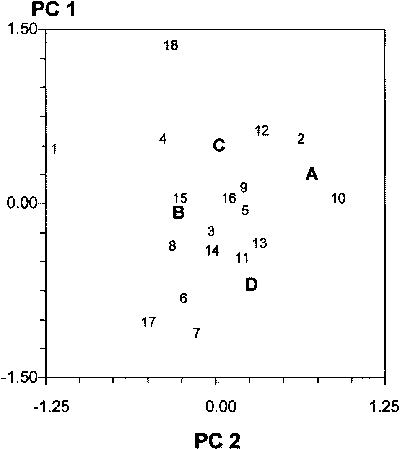
Source: Annicchiarico and Perenzin, 1994.
Estimation and test of model parameters
For the definition of an AMMI analysis table, the GL interaction SS in the ANOVA is divided into portions relating to each significant PC axis and to a residual term. The SS for each PC can be obtained as the proportion of GL interaction variation accounted for by its eigenvalue (which is unaffected by the definition of genotypes or locations as individuals in the analysis) multiplied by the ANOVA GL interaction SS. According to Gollob (1968) the DF for the PC axis n can be calculated as:
DF = g + l - 1 - 2 n
where g = number of genotypes and l = number of locations. The GL interaction SS and DF not accounted for by significant PC axes are pooled in the residual term. An MS can then be calculated for each PC and the residual. The procedure may be verified for data in Table 4.4. The proportion of variation explained by eigenvalues is 0.22 for PC 1 and 0.16 for PC 2, while the model R2 is 0.22 + 0.16 = 0.38 = 38%. For example:
PC 2 SS is 0.16 × 587.9 = 94.1
PC 2 DF is 18 + 31 - 1 - 4 = 44
Statistical testing of PC axes has mainly been investigated for analysis of a GE interaction matrix (applicable to GL interaction analysis for trials not repeated in time). An early F test devised by Gollob (1968) is too liberal (biased towards too many significant results) both in theory and on the basis of simulation results (Mandel, 1971; Cornelius, 1993). Cornelius (1993) proposed the FGH2 test, using approximations published in an earlier paper (Cornelius, 1980), as well as the FGH1 test and some simulation tests that are expected to produce results very similar to the FGH2 test while requiring more extensive calculation. In addition, Cornelius et al. (1992) described an alternative test: the FR ratio. Simpler to calculate, FR is more robust in the presence of heterogeneous within-site experimental errors than the FGH2 test (Piepho, 1995). Gauch (1988, 1992[13]) proposed a further test criterion based on a cross-validation procedure. The available plot values (replicates) for each genotype-environment combination are randomly split into modelling and validation data, and the possible AMMI models (from AMMI-0 to AMMI-F) are compared in terms of predictive ability (i.e. the ability to explain variation in data not used in constructing the model itself). Following assessment, the selected AMMI model is reparametrized using information from all data. For trials in randomized complete block designs, Piepho (1994a) recommends splitting complete blocks within environments rather than single replicates, in order to avoid the bias towards too few significant PC axes caused by an error term inflated by the block effect. Nevertheless, this test tends to be too conservative because modelling relies on a subset of the available data, which is less accurate than modelling all data (as performed after model choice) and is therefore somewhat biased towards simpler, lower-ranking AMMI models (Cornelius, 1993). Finally, Gauch (1992[14]) suggests a simple guideline for model selection based on the estimation of the noise level expected in the GE interaction matrix.
The application of most of the above tests to AMMI analysis of GL interaction for trials repeated in time is discussed by Annicchiarico (1997b). For cross-validations, two procedures are proposed, aimed at eliminating undue sources of variation from the relevant error term in the context of ANOVA models in Table 4.2. For the application of the remaining criteria it is necessary to utilize the appropriate error term for GL interaction - i.e. GLY interaction (Table 4.2) or GY interaction within locations (Table 4.3) - rather than the pooled error term (which is applicable in the absence of repetition in time). Although the preferred testing procedures may vary according to the size of the GL matrix and the number of test years (Annicchiarico, 1997b), the adoption of the FR test can be recommended in a wide range of situations (also because of its simplicity and robustness).
The FR test verifies the significance of the residual GL interaction variation in each AMMI model, beginning with AMMI-0. By an ordinary F ratio, the MS of the residual is tested on the same MS used as the error term for the GL interaction in the ANOVA. A significant result implies the addition of one more PC to the model (i.e. the significance of the newly-added PC). The test for PC 1, in which the residual is represented by the entire GL interaction, coincides with the ANOVA F test for the interaction. For example, consider the test for PC 2 in Table 4.4. For the residual GL interaction from AMMI-1:
SS is 587.9 - 129.3 = 458.6.
DF are 510 - 46 = 464.
MS is 458.6/464 = 0.99.
Therefore, PC 2 is also admitted in the model. The main drawback of the FR test is that no PC 1 can be declared significant in the absence of significant GL interaction, even if it accounts for most of the GL interaction SS. In such a rare event, reported by Zobel et al. (1988) for one data set, the signal-to-noise ratio criterion is prone to the same drawback; more complex tests, such as FGH2, should therefore be envisaged.
AMMI analysis is aided by adopting customized statistical software (including IRRISTAT, see Section 5.9). When such software is not available, two separate principal components analyses must be executed on the GL interaction matrix. The analyses consider genotypes or locations in turn as individuals and original variables. Location and genotype scaled scores on the PC axis n can be obtained from their respective eigenvectors issued by the two analyses, multiplied by the square root of the relevant singular value (√ ln). Alternatively, the scaled scores can be obtained from the original scores of locations and genotypes on PC n, dividing by √ ln. In both cases, ln can be calculated from the eigenvalue ln2, which is equal to the GL interaction SS accounted for by PC n in the AMMI analysis, expressed on a genotype by location cell mean basis by dividing by N' (where N' = no. test years [or crop cycles] x no. experiment replicates). Considering 10 genotypes grown in 20 locations in trials with 3 replicates conducted over 4 years, if the ANOVA GL interaction SS is 256.9, and the proportion of GL variation explained by PC 1 is 0.274:
l12 = (0.274 × 256.9)/(4 × 3) = 5.866
√ ln = (l12)0.25 =1.556
location (or genotype) PC 1 scaled score = location (or genotype) eigenvector × 1.556
location (or genotype) PC 1 scaled score = location (or genotype) original score/1.556
The last of these equations may also be used to obtain original scores of locations, of possible interest for site classification performed by cluster analysis (discussed below), when using specific software providing scaled PC score values.
The performance of two independent principal components analyses the additional problem of a potentially wrong sign of the genotype or the location eigenvectors, assigned independently in the two analyses. The polarity of eigenvectors and PC scores is arbitrary in AMMI analysis, but pairs of genotype and location scores must possess the same sign (positive or negative) to produce a positive GL interaction effect, and different signs to produce a negative GL effect. Therefore, signs of eigenvectors and PC scores may need to be inverted for genotypes (or locations), following the comparison between modelled and observed GL interaction effects. Several genotype-location pairs possessing the highest scores (in absolute terms) on the PC axis reveal the sign of the observed GL effect. The correct sign provides the best match between modelled and observed effects.
Modelled yield responses and cultivar recommendations
The expected yield response (Rij) of the genotype i in the location j is (according to the selected AMMI model):
Rij = m + Gi + Lj + ∑ (uin √ ln) (vjn √ ln) =m + Gi + Lj + ∑ (uin' vjn')
where m is the grand mean, Gi and Lj are the main effects for the genotype i and the location j, uin' = (uin √ ln) indicates the scaled score on the axis n for the genotype and vjn' = (vjn √ ln) that for the location. Since changes in genotype rank across locations only depend on the multiplicative term, the adaptive responses can conveniently be represented as a function of the scaled scores of locations on the statistically significant PC axes. The location main effect has no influence on genotype value and it complicates the graphic representation of adaptation patterns. Gauch (1992) and Gauch and Zobel (1997) therefore proposed to eliminate this effect from modelling by representing the expected yield responses in terms of nominal yields. This has the additional advantage of simplifying the calculations. For an AMMI-1 model, the nominal yield (Nij) of the genotype i in a given location j can be estimated from the genotype mean value (mi) and the scaled scores of genotype and location on PC 1:
Nij = m + Gi + (ui1 √ ll) (vj1 √ ll) =mi + (ui1' vj1')
[5.4]
The nominal yield responses of genotypes may be represented by straight lines as a function of location PC 1 scores reported in abscissa. This is shown in Figure 5.4 (A) for seven lucerne varieties grown in ten locations in northern Italy (the lowland sites in Annicchiarico [1992]). For each genotype, nominal yields are simply calculated for the two locations with extreme PC 1 score values (sites 'p' and 'o') and the two values connected by a straight line. On the basis of adaptive patterns:
'La Rocca', 'Prospera' and (to a lesser extent) 'Robot' can be recommended for the area represented by sites 'p' and 'l';
'Prosementi' and (to a lesser extent) 'Garisenda' and 'Robot' are preferable in a vast area, including sites 'z', 'a', 'b', 's' and 'e'; and
'Orchesienne', 'Europe' and (to a lesser extent) 'Prosementi' are the best-performing in the area comprising sites 'u', 'o' and 'c'.
Note: Site classification based on cluster analysis of site scores on PC 1 (see Fig. 5.7 for geographic position of coded locations).
Source: Annicchiarico, 2002.
These subregions are similar to those summarized in Figure 5.4 (A) representing the cluster analysis site classification based on GL effects for all cultivars (discussed below also in geographical terms). Incidentally, in subsequent trials, recommendations allowed for higher yields (6% in the first and 3% in the third subregion) than those widely recommended (on the basis of average yields of genotypes across sites) (Annicchiarico, 1998). The extension of results to new locations is less straightforward for AMMI modelling than for joint regression, because it cannot be based on a definite site characteristic, such as mean yield. In general, the response of a new site is expected to be similar to that of the closest test site, on the basis of a supposedly close relationship between similarity for GL effects and geographical proximity. However, additional information on environmental factors related to GL interaction may greatly facilitate the characterization of subregions and the spatial and temporal scaling-up of results (see Section 5.8, in relation to subregion definition for genotype recommendation and breeding).
An indication of the extent of statistical differences between varieties on varying sites score on PC 1 in a graph like Figure 5.4 (A) can be provided by the mean value of Dunnett's one-tailed critical difference calculated in a similar way to joint regression. An appropriate error term is represented: by the average GY interaction within locations (obtained, for ANOVAs with the time factor crossed with location, by pooling SS and DF values of GY and GLY interactions) for trials repeated in time, and by the pooled experiment error for trials not repeated in time. The latter applies to Figure 5.4 (A), where: Merr = 4.09; t' ≈ 1.79 (Table 4.6) for P < 0.20 and p = 10 (eleven cultivars overall, of which seven are shown); N = no. replicates = 4; and mean critical difference d ≈ 1.79 √ (2 × 4.09/4) = 2.56 t/ha. This value, superimposed on yield responses in Figure 5.4 (A), would slightly enlarge the range of recommended material. The critical difference is potentially valid also for comparison of nominal yields in AMMI models of higher complexity.
For specific recommendation on each site also, indications based on genotype comparison at the conventional P < 0.05 rate of Type 1 error may have negative implications due to concurrently high Type 2 errors. For example, recommending the AMMI-modelled best-yielding set of varieties based on Dunnett's one-tailed critical difference at P < 0.05 (average of five varieties) has on average provided over 3 percent lower yields than merely recommending the top-ranking variety (for data sets in Table 3.1, using 4 years for modelling and 2 other years for verification of yield gains - Annicchiarico, unpublished results).
For an AMMI-2 model, nominal yields can be estimated from the genotype mean value (mi) and the product of genotype and location scaled scores on PC 1 and PC 2:
Nij = mi + (ui1' vj1') + (ui2' vj2')
[5.5]
The graphical definition of mega-environments based on best-yielding material is complicated by the difficulty of representing the genotype responses as a function of site scores on two PC axes simultaneously. After representing the site scores as points in the bidimensional space of PC 1 and PC 2, a third dimension is required to represent the yield levels. However, the "winning" genotype expected for each location can be determined by calculating AMMI-2 nominal yields, and locations with the same best-yielding genotype can be grouped into the same subregion. For example, the definition of subregions and best-yielding material on the basis of repeated testing of 10 bread wheat varieties in 20 Italian locations (Annicchiarico et al., unpublished results) is reported in Figure 5.5 (A). Genotype '7' may be recommended on 12 sites, and cultivars '2', '3' and '4' on a small number of sites. Despite the small number, a specific recommendation (giving rise to a four mega-environment scenario) may be justified. The straight lines - subdividing the 20 coded locations into four subregions and defining boundaries in which the winning genotypes of two adjacent subregions have the same expected yield - can be calculated using appropriate software (see Section 5.9). The graph can also help in assigning new locations to subregions (see Section 5.8). However, it is possible to group sites merely on the basis of similarity of winning genotypes. If genotype recommendation considers more than one cultivar per subregion, sites can be grouped on the basis of the same two (or more) best-yielding genotypes. For estimation of nominal yields in AMMI-3 models, the product of genotype and location scaled scores on PC 3 is added to the terms in equation [5.5]. Estimated parameters for higher-order PC axes are also included for AMMI models of increasing complexity.
The present approach for modelling GL effects and defining subregions for genotype recommendation from trials repeated in time differs from that proposed by Gauch (1992[15]), because it is based on the mean response of locations for GL effects. The results are thus simplified (e.g. the 20 points for locations in Fig. 5.5 [A] would become 80 for results expressed for individual environments). The average inconsistency of locations for GL effects (i.e. GLY interaction) is taken into account by the error term adopted for assessing the GL interaction effects. For a relatively low number of test sites, the results of an additional AMMI analysis performed on GE effects may reveal whether or not a location is characterized by unusual variation for PC scores between its environments, leading to inconsistency of the winning genotype between years (or crop cycles) (Fig. 6.5 in Gauch, 1992[16]). However, a reliable assessment of the frequency of different winning genotypes in each location (i.e. the information required for recommendation in this context) may be difficult when based on the limited number of test years (< 3) normally available. This approach is difficult to apply when more than one recommended genotype is considered for each site.
Location classification for breeding
The provisional definition of subregions for breeding requires that site classification be based on similarity for overall GL effects (Table 5.1). The performance of cluster analysis, using as variables (i.e. dimensions in an Euclidean space) the scaled or unscaled scores of sites on the significant PC axes, means that the noise portion of GL interaction - which tends to be pooled into the non-significant, residual GL interaction term - may be substantially eliminated from the assessment. This procedure is consistent with one of the major objectives of ordinary principal components analysis, namely, summarizing the information provided by many correlated original variables (each one corresponding to the set of GL effects of genotypes in a given location) into a few uncorrelated PC variables, thus simplifying the multivariate comparison of the individuals (in this case, locations). In this context, the assessment of site similarity based on original rather than scaled PC scores of sites (e.g. Annicchiarico, 1992; Annicchiarico and Perenzin, 1994) may be preferable when there are two or more PC axes (while scaling does not affect assessment based on PC 1 scores only). Ward's incremental SS or the average linkage methods (with a squared Euclidean distance as the dissimilarity measure) can again be recommended for cluster analysis. When applied to PC axes, the dissimilarity measure for cluster analysis requires no prior standardization of variables, because the variation in site score on each PC axis is proportional to the importance of each variable (Dagnelie, 1975b[17]; Afifi and Clark, 1984[18]). As mentioned above, Ward's method is particularly suited to the truncation criterion based on the significance of the within-group GL interaction in ANOVAs.
For example, consider the cluster analysis applied to PC 1 scores of nine locations (all except site 'e') in Figure 5.4 (A). Results of site grouping for the final fusion stages are reported in Figure 5.6, together with significance levels for the within-group GL interaction according to ANOVA. P levels < 0.01 require further subdivision of groups, whereas higher P levels are here acceptable for group definition (as GL interaction is tested on a relatively small error term, i.e. the pooled experimental error). Three groups of locations may be defined in the analysis. They are superimposed (as subregions A, B and C) on the ordination of sites in Figure 5.4 (A). In the report by Annicchiarico (1992), location 'e' was actually represented by two environments clustered, respectively, in subregions B and C, implying a border position between these subregions. The results of site classification, combined with information on environmental factors related to the occurrence of GL interaction (Annicchiarico, 1992, 2000), have allowed for the geographical definition of potential subregions reported in Figure 5.7 - confirmed by AMMI and the cluster analysis results obtained for an independent set of subsequent trials (Annicchiarico, 2000). Predicted yield gains from different selection strategies, as well as opportunities for selection in artificial environments, are further discussed in Section 6.1.
Results of location classification for the bread wheat example based on: cluster analysis of PC 1 and PC 2 site scores as original variables; an average linkage method; and P > 0.05 for the within-group GL interaction as a truncation criterion for definition of groups of locations, are given in Figure 5.5 (B). In this case (unlike the lucerne example) the preliminary definition of mega-environments for breeding is distinctly different from that for variety recommendation (Fig. 5.5 [A]). The provisional subregions 1 and 2 are large enough to justify specific breeding (Fig. 5.5 [B]), whereas subregions 3 to 5 (represented by one location each) are too small and can be merged with subregion 1 (the closest). The site classification is geographically meaningful: the provisional subregion 2 groups locations in southern Italy, while the larger subregion 1 groups sites in northern and central Italy.
Figure 5.6 - Cluster analysis
of test locations performed on site scores on the first GL interaction PC axis,
using the lack of significant (P < 0.01) GL interaction within
group of locations as the truncation criterion for definition of
groups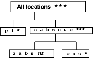
Note: * = P < 0.05; *** = P < 0.001 (see Fig. 5.4 for PC scores and Fig. 5.7 for geographic position of locations).
Source: Annicchiarico, 2000.
For AMMI-1 models, an alternative criterion of site classification for breeding purposes can be provided by estimating the main crossover point for nominal yields of genotypes modelled as a function of the site scaled score on PC 1, to be used as a cut-off for the definition of two subregions. The procedure proposed is an extension to AMMI analysis of the procedure developed by Singh et al. (1999) for joint regression. The main crossover point Xco in formula [5.3] relates to genotype slopes which vary around a zero mean (bi - 1 = βi) and are different for intercept value ai (i.e. nominal yields that have zero grand mean and are expressed as a function of site mean yield). A similar formula can be obtained for AMMI nominal yields expressed as in Figure 5.4, after performing a double change of origin that causes the zero value for the abscissa and the ordinate axes to coincide with the lowest site score on PC 1 and the grand mean, respectively.
The slope of the genotype i as a function of PC 1 can be expressed as:
βi = (Ni2 - Ni1)/(v21' - v11')
where j = 1 is the location with the lowest PC 1 score; j = 2 is the location with the highest PC 1 score; v11' = (v11 √ l1) and v21' = (v21 √ l1) are the scaled scores on PC 1 for these locations, as expressed in the graph; and Ni1 and Ni2 are the nominal yields of the genotype i on the site with lowest and highest PC 1 score, respectively (these values are already calculated for the graphical expression of adaptive responses).
The main crossover point expressed in the same PC 1 score units as in the graph can be estimated as:
Xco = (-∑ ai βi/∑ βi2) + v11' = (-∑ ai βi/∑ βi2) - | v11'|
[5.6]
where ai = (Ni1 - m) is the intercept value for the genotype i.
For the lucerne example in Figure 5.4 (A), Xco = -0.19 (calculated over 11 cultivars). Therefore, the coded locations 'p', 'l', 'z', 'a' and 'b' would be assigned to one subregion and the remaining sites to another subregion. While only two groups of locations can be defined by this approach, three or more groups may be defined by the shifted multiplicative model (Crossa et al., 1993, 1995) based on crossover GL effects.
Concluding remarks
AMMI analysis does not provide a direct explanation for the occurrence of GL interaction, since environmental variables are not included in the model. However, values of these variables for sites where they are available can be related to site scores on significant PC axes by correlation or regression techniques. It is thus possible to distinguish the environmental factors likely to play a major role in this context (Annicchiarico and Perenzin, 1994; van Eeuwijk, 1995; Bidinger et al., 1996). Such external information - which may be incorporated into biplots of PC 1 and PC 2 axes (van Eeuwijk, 1995) - can contribute to subregion characterization and scaling-up of results (see Section 5.8). Likewise, morphophysiological traits of genotypes (even if recorded in a small number of sites), averaged across observations for each entry, can be used for correlation analysis with estimated parameters of genotype adaptation (i.e. significant PC scores and mean yields) in order to highlight characters associated with specific or wide adaptation (see Section 6.3). Correlation results for sites and genotypes are expected to be consistent with each other. For example, if the ordination of sites on PC 1 has high positive correlation with rainfall, the ordination of genotypes on the same axis probably reveals positive correlation with lateness of flowering (or crop cycle) and/or negative correlation with physiological indicators of drought resistance, as mechanisms of drought escape and resistance may produce specific adaptation to low rainfall (i.e. low PC 1 score) sites. In joint regression analysis, environmental variables and adaptive traits associated with the occurence of GL interaction may be revealed, respectively, by correlation of site mean yield with environmental variables and by correlation of regression slope with morphophysiological traits of genotypes.
Early models of genotype regression on environmental factors are proposed by Shukla (1972a) for one environmental covariate, and by Hardwick and Wood (1972) for two or more covariates in a multiple regression approach. Applications of these methods, mostly targeted to analysis of GE rather than GL effects, are reported by Wood (1976), Saeed and Francis (1984), Kang and Gorman (1989), Piepho et al. (1998) and others. One development of this technique has involved the simultaneous use of environmental and genotypic covariates, as proposed by Denis (1980 and 1988) and applied by Biarnès-Dumoulin et al. (1996), Balfourier et al. (1997) and others. Regressions are usually linear, although quadratic terms may also be included as additional covariates in the multiple regression model (e.g. Saeed and Francis, 1984).
Factorial regression is considered herein for models including only environmental covariates. The interaction effects GLij are modelled as a function of the mean value (Vjn) on the site j of the environmental variable n. If βin represents the regression coefficient of the genotype i on the covariate n:
GLij = αi + ∑ βin Vjn + dij
where αi is the intercept value for the genotype and dij is the deviation from the model. For one environmental variable equal to site mean yield, the model coincides with Perkins and Jinks' joint linear regression. Positive β values are indication of a good response to sites with a high level of the environmental variable concerned, while negative values indicate a good response to sites with a low level of variable. Specific adaptation to these sites implies relatively high values of the other adaptation parameter: genotype mean yield. Qualitative covariates (e.g. soil type) may be used, but information must be incorporated through a set of dummy variables (Piepho et al., 1998).
Estimation and test of model parameters
The factorial regression model is constructed with the progressive addition of the most important covariates (Denis, 1988). In the absence of powerful or specific statistical software (see Section 5.9), the best one-covariate model may be identified on the basis of the proportion of GL interaction SS accounted for, i.e. the model R2, using procedures similar to those described for joint linear regression. There are two possible procedures:
the model SS relating to regressions of GL effects for individual genotypes are summed up and expressed as the proportion of the total SS in the regressions; or
SS values for genotype regressions and deviations from the model (or residual GL interaction) are obtained as the model and error SS, respectively, in an analysis of covariance of all GL effects as a function of the genotype factor and the interaction of genotype with site mean value of the covariate.
Testing for statistical significance of the covariate (i.e. heterogeneity of genotype responses to the environmental variable) can be limited to the best model. For integration with ANOVA results in a factorial regression table, the SS for the covariate and the residual GL interaction need be multiplied by N' = no. test years (or crop cycles) × no. experiment replicates. Alternatively, they can be calculated by multiplying the model R2 (for the SS for the covariate) and its complement to one (for the residual GL interaction) by the ANOVA GL interaction SS. The GL interaction DF is partitioned into a (g - 1) portion for the covariate and a remainder for the residual. The MS for both terms can be tested on the appropriate error term for the GL interaction in the ANOVA (Saeed and Francis, 1984). An alternative error for the covariate term can be represented by the variation for the same error pooled with that of the residual GL interaction (Denis, 1988).
After identifying the best one-covariate model and verifying the significance of its covariate term, the best two-covariate model is found by comparing (on the basis of their R2) the possible multiple linear regression models including the best single covariate (previously identified). Model SS and R2 and residual GL interaction SS are obtained: by summing the results of multiple regression analyses of GL effects executed for individual genotypes; or through an analysis of covariance of all GL effects including, in addition to the genotype factor, a genotype × covariate site mean value interaction term for each of the two environmental variables. Testing of the second covariate (limited to the best two-covariate model) relates to the portion of GL interaction SS explained by its addition, i.e. the partial regression SS, calculated as the difference in model SS between the two-covariate and the best one-covariate model (multiplied by N' = no. test years [or crop cycles] x no. experiment replicates, for inclusion in the factorial regression table). Alternatively, the partial regression SS may be calculated as the difference in R2 between the two-covariate and the one-covariate model, multiplied by the ANOVA GL interaction SS. The DF accounted for by the second (and additional) covariate(s) are always (g - 1). If the MS of the added covariate (tested as for the first covariate) is significant, the best three-covariate model can be searched for, and the significance of the last entered variable verified (and so forth, for models of increasing complexity, following a forward selection strategy). Otherwise, the best one-covariate model is retained (if its covariate is significant).
The estimation and testing of parameters of genotype adaptive response, obtained either from analysis of the single genotypes or from analysis of covariance (in which αi and βin values are estimated by parameters for, respectively, the genotype and the interaction of genotype with site mean value of the covariate n), can conveniently be considered only in relation to the selected factorial regression model. Testing of each βin value for difference to zero in relation to deviations from the model of the genotype i (as obtained by individual analysis) is somewhat more reliable than testing in relation to an average value of deviations (as provided by analysis of covariance).
Factorial regression performed on original yields rather than GL effects (a procedure so far not considered) would inflate the GL interaction component accounting for deviations from the model. This source of variation would include the lack of fit not only of individual genotype regressions but of site mean yield (the latter would be responsible for the increase or decrease of all observed genotype yields relative to regressions, whenever the mean yield response of a site to the environmental variable(s) deviated from a linear response). However, this procedure may be useful for predicting genotype responses from information provided by historical, largely unbalanced data sets. In this case, estimating genotype main effects may prove difficult. Therefore, mean yield and GL interaction effects could be estimated (separately for each genotype) by means of a stepwise multiple regression analysis of original yields as a function of the available site covariates. It is very unlikely, however, that the same environmental variables will be selected for all genotypes (thereby increasing the complexity of modelling).
Modelled yield responses and cultivar recommendations
The expected yield of the genotype i in the location j is, according to the selected factorial regression model:
Rij = m + Gi + Lj + αi + ∑ βin Vjn
where m is the grand mean and Gi and Lj are the main effects for the genotype i and the location j, respectively. Modelling is reliable in the range of observed covariate values, and estimates of parameters should be kept in the model even when they are not statistically significant. As for AMMI analysis, the expected yield responses can be expressed in terms of nominal yields (Nij) to simplify their calculation and, possibly, their graphical expression.
Nij = mi + αi + ∑ βin Vjn
[5.7]
where mi is the mean value of the genotype i.
In the graphical expression there are problems and opportunities similar to those for AMMI analysis. When genotype adaptive responses can be modelled in one dimension as a function of the only covariate in the model, nominal yields can be represented by straight lines (connecting their values - calculated only for the extreme covariate levels in the graph), as reported in Figure 5.1 (B) for response to site mean rainfall (from January to June) of the same cultivars already modelled by joint regression (Fig. 5.1 [A]). Straight lines are not adequate for modelling actual yields (by addition of site main effects), unless the response to rainfall of site mean yield is perfectly linear. The comparison of joint regression and factorial regression results reveals some inconsistency (as is normal for different models). In particular, 'D 3415' is never top-yielding in the range of site mean rainfall (Fig. 5.1 [B]). Specific genotype recommendation may be envisaged for two subregions:
relatively low mean rainfall (< 400 mm), where 'Messapia' is the preferable cultivar; and
relatively high mean rainfall (> 400 mm), where 'Karel' and 'W 4267' are preferable.
Multiple comparison among genotypes at different rainfall values may be performed by means of Dunnett's one-tailed critical difference, as described for joint regression (the error term for the test - when the residual GL interaction is not significant - is the GY interaction within locations in the presence of repetition in time of the trials, and the pooled experiment error in the absence of repetition in time). The critical difference may also be calculated for models with two or more environmental covariates.
The graphical expression of genotype responses for a two-covariate scenario is more complex and requires a bidimensional representation of best-yielding genotypes as a function of site values for the covariates. Figure 8.3 in Section 8.3 provides an example of outputted information with the expected pair of top-yielding genotypes for each combination of 10 rainfall by 10 winter temperature levels of sites. Combinations (represented as cells) with the same winning genotypes can be grouped together. The graph requires the preliminary estimation of nominal yields of the genotypes (usually a subset of better-yielding entries, to avoid extensive calculations) for each pair of covariate values according to equation [5.7]. A denser grid of points in Figure 8.3 (e.g. formed by the combination of 20 rainfall by 20 temperature values) allows for a more fine-tuned definition of winning genotypes. The spatial and temporal scaling-up of results is straightforward by the factorial regression approach, depending on the site mean value of the significant covariates. Subregions are defined, grouping locations with same best-yielding material.
Piepho et al. (1998) propose an alternative procedure for genotype comparison at different covariate levels, considering possible differences between components of the error term as they may occur for specific pairs of compared genotypes. Although more appropriate, this approach requires more complex calculation, as error terms are estimated for each considered pair and different factorial regression models may need to be adopted, depending on the value of the site(s) of specific interest.
Location classification for breeding
For preliminary definition of subregions for breeding, factorial regression analysis may be complemented by hierachical cluster analysis performed on site values of the significant environmental covariates. Analysis may also include non-test sites in the target region for which data on the relevant environmental variables are available; results are thus scaled up to new sites. The temporal scaling-up of results can be obtained by inputting long-term rather than test year data of relevant climatic or biotic variables. Earlier recommendations concerning the clustering method and the dissimilarity measure may also be applied. However, the inclusion of new sites or long-term data makes the truncation criterion based on the level of within-group GL interaction more difficult to apply and less reliable. An average linkage clustering strategy (more useful for detecting true discontinuities among locations, although less useful for minimizing the within-group GL interaction - DeLacy et al. [1996a]) is the most appropriate in this context.
Refinement of the cluster analysis technique that usually requires a modest increase in the calculations is represented by the assignment to each environmental variable of a weight proportional to its importance in the factorial regression model, as suggested (in a slightly different context, i.e. modelling of site mean yield) by Brown et al. (1983). The weight is proportional to the partial regression SS of each environmental variable in the selected factorial regression model. The SS value may be calculated as the difference in SS between the regression model with the considered covariate and the regression model without it (all other significant covariates being included). The assessment requires: no additional multiple regression analysis for a two-covariate selected model; one additional multiple regression analysis (excluding the best single covariate) for a three-covariate selected model; etc. For the application of weights, the standardization of each variable to a standard deviation value proportional to its weight is recommended. For example:
considering three covariates V1, V2 and V3 with, respectively:
- partial regression SS of 50, 30 and 20
- estimated standard deviation of s1, s2 and s3
and assigning a unity weight to the least important variable:
- the respective weights are 2.5, 1.5 and 1; and
- the standardization for a given site j is obtained by the variable
transformations:
V'j1 = Vj1 2.5/s1
V'j2 = Vj2 1.5/s2
V'j3 = Vj3/s3
For factorial regression models including only one covariate, the estimation of the main crossover point for genotype nominal yields modelled as a function of the covariate value can provide an alternative criterion for the preliminary definition of two subregions for breeding based on the test locations. Extending Singh et al. (1999)'s approach to factorial regression - as was done for AMMI modelling - nominal yields as expressed in Figure 5.1 (B) can be submitted to a double change of origin, whereby the zero value for the abscissa and the ordinate axes coincides with the lowest site mean value of the covariate and the grand mean, respectively. The slope of the genotype i as a function of the covariate V1 is coincident with that expressed by the bi1 value in formula [5.7]. The main crossover point expressed in the same covariate units as in the graph can be estimated as:
Xco = ( - Σ ai βi / Σ βi2) + V11
[5.8]
where V11 is the lowest site value for the covariate; ai = (Ni1 - m) is the intercept value for the genotype i in the current formulation (which is different from αi in formula [5.7]); and Ni1 is the nominal yield of the genotype at the value V11 of the covariate.
In Figure 5.1 (B), Xco = 251 mm (calculated over 9 cultivars included in the study). The crossover point can also be used for assigning new locations to subregions, depending on the site mean value of the covariate.
Concluding remarks and comparison of models
Sometimes, just one or two environmental covariates can explain a remarkable portion of GL interaction variation (Saeed and Francis, 1984; Biarnès-Dumoulin et al., 1996; Giauffret et al., 2000; see also case study in Chapter 8). However, careful selection of environmental variables, on the basis of common sense and their putative importance on adaptation patterns, is recommended prior to analysis - in order to both limit the calculation process and avoid the risk of multicollinearity problems. Such problems may occur when several highly correlated variables are considered simultaneously. Multicollinearity, which may lead to dangerously unstable predictions, may be eliminated by adopting a partial least squares regression model (Talbot and Wheelwright, 1989; Vargas et al., 1998). Vargas et al. (1999) report agreement between the results of this technique and those of factorial regression for a data set including a very large number of environmental variables; this suggests, however, that multicollinearity may be a minor problem in a wide range of situations. On the other hand, a reduction in the dimensions for the factorial regression model sought via the reduced rank factorial regression approach may sometimes prove unfeasible (van Eeuwijk, 1992). Although more complex, both these alternative regression techniques offer the additional advantage of a highly informative graphical output (Aastveit and Martens, 1986; van Eeuwijk, 1992).
Compared to joint regression and AMMI analysis, factorial regression allows for an explicit assessment of the relationships of environmental variables with GL effects. Our understanding of the reasons contributing to GL interaction (both in general and for individual genotypes - as depicted by estimates of β coefficients) is thus improved. The information generated facilitates the characterization of subregions and the spatial and temporal scaling-up of results (see Section 5.8), as well as the identification of genetic resources with definite response to key environmental factors. This technique, however, requires the availability of data for major environmental variables in the complete set of test environments, a condition that may severely limit its application. Conversely, with AMMI or joint regression modelling, locations with missing environmental data can be excluded from correlation or regression analyses assessing the relationships of these variables with GL effects, but used for modelling yield responses. In various reports (van Eeuwijk and Elgersma, 1993; Vargas et al., 1999; see also case study in Chapter 8), AMMI and factorial regression identify the same environmental factors as those related to GL interaction occurrence, producing similar results in terms of genotype adaptive responses and site similarity for GL effects, despite the higher requirements in terms of factorial regression input data.
Factorial regression models including genotypic covariates allow for proper statistical assessment of the relationships of adaptive responses with morphophysiological traits that are recorded in all environments (Denis, 1988; van Eeuwijk et al., 1996). However, correlation of genotype values for these traits (the average of observations from even a small number of sites) with values of β coefficients may provide indication of the traits involved in the response to each environmental covariate (see Section 6.3). Correlation results are expected to be in logical agreement with the covariate concerned (e.g. longer crop cycle positively correlated with β values for response to rainfall amount).
A word of caution is required with respect to the identification of causal factors for GL interaction. An environmental variable - either significant as a covariate in the factorial regression model or significantly related to site ordination on significant PC axes - may be correlated with an unmeasured causal factor rather than representing a causal factor itself. This may be evident (e.g. site altitude, underlying the effect of low temperatures at some growth stages) or obscure (e.g. soil pH, possibly hiding the effect of soil aluminium as the unmeasured, correlated causal factor). Similarly, putative adaptive traits as identified by the analyses (see Section 6.3) may be genetically correlated with the actual adaptive traits. Moreover, sampling errors may underemphasize the importance of environmental or genotypic variables (especially when modelling does not contemplate the use of these variables). However, false assumptions regarding causal factors do not necessarily have a very negative impact. For example, the exploitation of site altitude as an environmental variable for scaling up the results of subregion definition for breeding or variety recommendation (see Section 5.8) may be effective if the variable is highly correlated with the underlying causal factor (e.g. low temperatures). On the other hand, specific breeding for a subregion characterized as having low soil pH, based on artificial screening for tolerance to low pH, is largely ineffective if the real causal factor for GL interaction is soil aluminium. Indications of causal factors can often be verified with small ad hoc experiments.
When different analytical models have been applied to the same yield data (with possible different indications), it must be asked which approach is the most reliable. Model comparison is sometimes based on model R2 (i.e. the portion of GL interaction SS accounted for by significant GL interaction parameters in the model). This criterion (which focuses on model accuracy with respect to the same data that generated the model itself) fails to recognize that model parsimony (expressed by low number of DF) is a desirable characteristic contributing to the ability to predict genotype performance in a novel, independent data set (Gauch, 1992[19]). For example, compared to AMMI-1, the joint regression model is mathematically incapable of accounting for more GL interaction SS, while accounting for less DF. Comparison of models in terms of MS value takes into account accuracy and parsimony, but is only appropriate for models with one parameter (joint linear regression; AMMI-1; factorial regression with one covariate). Brancourt-Hulmel et al. (1997) propose a general measure of model quality provided by the ratio:
% GL interaction SS/% GL interaction DF
for SS and DF values accounted for by the significant parameters in the model.
An alternative criterion for model comparison may relate to the estimated variance of the significant parameters. The variances of PC axes are summed up because the principal components are uncorrelated (which means that they add independent pieces of information). Similarly, the variance of any additional environmental covariate may be added to that of the first covariate as it relates to partial regression SS, i.e. independent information. If Becker's (1984) procedure for estimation of the heterogeneity of genotype regressions variance component is extended to PC axes or environmental covariates, the following formulae may be used for ANOVA models 1, 2 or 3 in Tables 4.1 through 4.3 (with the same formulations used in the tables):
|
|
SC2 = (MC - M5)/rl |
(for models in Table 4.1) |
|
|
SC2 = (MC - M8)/ryl |
(for models in Table 4.2) |
|
|
SC2 = (MC - M6)/ryl |
(for models in Table 4.3) |
where the MS of a given component of the GL interaction is indicated by MC and the estimated variance is indicated by SC2. For example, the variances of genotype regressions, PC 1 and PC 2 components of the GL interaction calculated from MS values of the ANOVA in Table 4.4 (according to the second formula) are 0.010, 0.007 and 0.005 (t/ha)2, respectively, indicating the superiority of AMMI-2 (0.012 [t/ha]2) over the joint regression model. The criterion proposed by Brancourt-Hulmel et al. (1997) would rather favour the regression model (% GL interaction SS % GL interaction DF = 0.104/0.033 = 3.15) over AMMI-2 (0.380/0.176 = 2.16), despite the very low amount of explained GL interaction (R2 = 10.4%).
Specific breeding is favoured by large genotype x subregion interaction and low GE interaction within subregions. Therefore, the MS ratio of these effects (calculated in the ANOVA including the factors: genotype, subregion and environment within subregions) may be used as an additional criterion for comparing different approaches for subregion definition in a breeding perspective. Especially in the absence of clear-cut indications, the estimation of yield gains predicted for each approach (see Section 8.2) provides an ultimate, fundamental criterion for comparison.
Adaptation patterns are herein investigated using a combination of ordination and classification techniques. There is ample literature providing method description (Williams, 1976b; Byth and Mungomery, 1981; DeLacy et al., 1996a) and documenting applications (Mungomery et al. 1974; Shorter et al., 1977; DeLacy et al., 1994, 1996c). The input data set is currently represented by a two-way matrix of genotype by location yield values (rather than GL interaction effects), averaged across years and/or experiment replicates. Yield data, however, are preliminarily standardized within-location to zero mean and unit standard deviation (by subtracting location mean yield and dividing by within-location standard deviation of genotype values). Standardization is recommended to remove the effects of site mean yield and heterogeneity of genotypic variance among locations from the assessment of site similarity for GL effects (Fox and Rosielle, 1982a; see also Section 5.6). Alternative techniques for classification of locations or genotypes, based on the analysis of a GL interaction data matrix, have been developed by Ramey and Rosielle (1983) and Lin and Butler (1988). An ordination technique, contemplating the execution of a principal components analysis on the genotype by location matrix of untransformed yields, is proposed by Yan et al. (2000), mainly as an alternative to AMMI analysis-derived procedures for the graphical display of the top-ranking genotype in each location.
Classification and ordination procedures
In its classification mode, pattern analysis implies the grouping of locations through a hierarchical cluster analysis based on site similarity in the Euclidean space represented by the standardized yields of genotypes. Classification usually also concerns genotypes, grouped together on the basis of similarity for GL effects and main effects, i.e. the adaptive response (as the standardization adopted does not remove the yield differences among genotypes, while compensating for a scale effect of individual locations on these differences [Yau, 1991]). A squared Euclidean distance as the dissimilarity measure and Ward's clustering method are normally recommended (DeLacy et al., 1996a; Cooper et al., 1996a). For site classification, a possible truncation criterion may be provided by the lack of significant GL interaction within a group of locations. However, alternative criteria are also available (DeLacy et al., 1996a).
Pattern analysis by the recommended procedure has the theoretical advantage of providing a grouping of sites that reflects the opportunities for exploiting indirect selection responses to locations, as these responses are maximized within potential subregions and minimized across subregions (Cooper et al., 1996a). Another advantage of this method over previous classification techniques is the rapidity of the analysis (no prior modelling of adaptive responses is required). A third advantage is its usefulness in the analysis of largely unbalanced data sets, using a procedure described by DeLacy et al. (1996b) (summarized below).
Cluster analysis following the modelling of GL interaction effects has the theoretical advantage of assessing site similarity after separating the pattern (retained in the significant GL interaction terms, such as PC axes or environmental covariates) from the noise portion of GL interaction variation. This advantage - confirmed in investigations by Crossa et al. (1991) and Smith and Gauch (1992) in relation to AMMI analysis - may produce in comparison with pattern analysis results: a poorer fit to the data observed (also in terms of predicted yield gain on the basis of the suggested definition of subregions); but a better prediction of actual, future responses of selected material. For pattern analysis, Crossa et al. (1991) therefore suggested using the expected yields of genotype-location combinations according to the selected AMMI model, rather than the observed yield values. This may be extended to the use of expected yields as provided by appropriate modelling through joint regression or factorial regression. Without ruling out this possibility, clustering locations according to the site characteristics that are directly associated with the occurrence of GL interaction (i.e. the mean yield, the score on significant PC axes or the value of significant environmental covariates: see Sections 5.2, 5.3 and 5.4) probably provides a faster and straightforward option for cluster analysis to complement joint regression, AMMI and factorial regression techniques.
Ordination of genotypes and locations in pattern analysis is performed by principal components analysis (Kroonenberg, 1995) or principal coordinates analysis (Gower, 1966; Mungomery et al., 1974) of the standardized data. It aims mainly to complement the cluster analysis results (e.g. by highlighting the response of individual sites or genotypes, or the extent of variation within the groups of sites and genotypes). The lack of integration with ANOVA results does not provide the user with an objective criterion for testing the significance of principal components and excluding the allegedly noise portion of GL effects from modelling of adaptation patterns. Indeed, the current modelling represents the standardized values observed, usually by means of a "performance plot" showing the mean performance of each genotype group averaged across sites of each location group (for the groups that are selected by cluster analysis). In addition, data standardization may introduce distortion to the modelled responses of genotypes (see Section 5.6). These characteristics make the previous analytical techniques preferable to pattern analysis when analysis is aimed at the targeting of genotypes. Therefore, pattern analysis is here envisaged mainly for site classification aiming at the definition of adaptation strategies. However, the opportunity offered by this technique for classifying genotypes according to their adaptive response may also prove useful in various breeding contexts (e.g. selection of breeding lines or identification of potential parent material), especially when the appreciation of these responses by graphs (such as Figs 5.1 or 5.4) is hindered by the large number of evaluated entries or the multidimensional adaptation pattern. Finally, contribution analysis (Shorter et al., 1977; DeLacy et al., 1996a) is an additional tool for obtaining insight into the relative contribution of individual test sites to GL interaction and genotype classification carried out by Ward's method.
Analysis of largely unbalanced data sets
The availability of largely unbalanced data sets composed of several historical data sets, each one relating to a specific year (or crop cycle) and having several test locations but few (or no) tested genotypes in common with the other data sets, is relatively frequent in multi-environment testing of breeding lines or commercial cultivars (especially where there is a high turnover of plant material). The combined analysis of this information for location classification may be realized using a procedure that requires different steps (DeLacy et al., 1996b):
estimation of the phenotypic correlations among test locations for genotype original yields in each individual data set;
averaging across data sets of the correlations for each pair of locations; and
transformation of the similarity matrix (as provided by correlation coefficients) into a dissimilarity matrix of squared Euclidean distances, inputting it (rather than the genotype by location matrix of standardized yields) into the cluster analysis.
Examples of this procedure are provided by DeLacy et al. (1994 and 1996c). Correlations based on fewer than four genotypes should not be considered. Averaging of correlations relative to the same pair of locations should be performed on values previously submitted to the z (inverse tanh) transformation, back-transforming to r the average z value (using tables provided in statistical textbooks: e.g. Steel and Torrie, 1960; Dagnelie, 1975a[20]). A weighted average should be used for correlations based on a variable number of genotypes, using the following formula (expressed for z values):
z = ∑ (ni - 3) zi/∑ (ni - 3)
where z is the weighted average, and zi and ni are the z value and the associated number of genotypes for the correlation, respectively, in the data set i. For example, the weighted average of the three phenotypic correlations r1 = 0 .50, r2 = 0.80 and r3 = 0.90, with the respective number of genotypes n1 = 16, n2 = 10 and n3 = 15, can be obtained through the z transformation as:
z = [(13 × 0.55) + (7 × 1.10) + (12 × 1.47)]/(13 + 7 + 12) = 1.01
which, once back-transformed, provides the average phenotypic correlation rp = 0.77 for insertion in the similarity matrix. Of course, pairs of locations may differ for number of correlations contributing to the average rp value, since some sites may be absent in some data sets. At least one individual correlation is needed for each pair of locations to allow both sites in the analysis. A higher number of individual correlations (e.g. 2) and more than four genotypes per correlation (e.g. 6-10) may be set as minimum values to increase the reliability of results. The transformation of the matrix of average correlations into the matrix of squared Euclidean distances (D values) among locations can be performed by transforming each rp value according to Gower's (1966) relationship (DeLacy et al., 1996a):
D = 2 (1 - rp)
The dissimilarity matrix relates to distances as they would be estimated on the basis of genotype yields standardized within location. A principal coordinates analysis is required for the possible ordination of locations in this case. By adopting appropriate, freely available software (see Section 5.9), it is possible to input the correlation matrix without any further calculation for execution of the cluster analysis. In this case, no truncation criterion based on the level of within-group GL interaction is available (as no combined ANOVA can be performed). Opportunities for subregion characterization and scaling-up of pattern analysis results are considered in Section 5.8.
Heterogeneity of genotypic variance
Data transformation in relation to heterogeneity of genotypic variance among environments (and in particular, locations) only concerns analyses aimed at the definition of adaptation strategies and yield stability targets. With special reference to pattern analysis of a genotype by environment matrix of yield data, Fox and Rosielle (1982a) proposed standardizing genotype values within environments, in particular to counterbalance the trend of high-yielding environments - supposedly characterized by higher variance of genotype values - having greater weight in the assessment of environment similarity for GE effects. Yau (1991) then showed that positive correlation of within-environment phenotypic standard deviation of genotype yields with environment mean yield is common in data sets characterized by large variation in mean yields. This correlation may occur because the variation in genotype yields is limited by the zero value in lowest-yielding environments. These indications can be extended to cluster analysis of locations based on site similarity for GL interaction effects, as it is substantially the case also for cluster analysis of PC scores of sites following AMMI modelling. In the presence of positive correlation between site mean yield (mloc) and within-location phenotypic standard deviation of genotype yields averaged across replicates (sp), higher-yielding sites are characterized by larger residuals from additivity (i.e. GL effects) and tend to show larger Euclidean distances from other locations. Conversely, low-yielding locations tend to be more similar than they really are in relation to genotype ranking. This is exemplified for the yield response of four hypothetical genotypes in four locations. Starting from responses in Data set A (sp constant), the effect of proportionality of sp with mloc is superimposed, resulting in Data set B (Table 5.2). This effect results in larger Euclidean distances of the highest-yielding site 'd' from the other sites, in comparison with distances for sp constant, with reference to the relevant dissimilarity matrix (i.e. that for GL effects) (Table 5.3). As a result, the highest-yielding site tends to cluster alone, while the remaining sites cluster together (data not reported). It can also be seen from the matrices of Euclidean distances relative to Data set A that the assessment of site similarity for GL effects based on original yields is biased by an effect of site mean yield (which inflates the distances between the sites with contrasting mean yield) even in the absence of proportionality between sp and mloc (Table 5.3). The within-location standardization of genotype values in Data set B (by subtracting site mean yield, and dividing by the within-site standard deviation of genotype values) can compensate for the proportionality of sp with mloc, providing Euclidean distances between sites (Data set E in Table 5.3) that coincide (in terms of relative differences) with those of Data set A. The distances assessed on genotype yields or GL effects coincide with standardized data (Table 5.3). Also two alternative data transformations, namely, the logarithmic one (Data set C in Table 5.2) and the division of genotype yields by site mean yield, i.e. the relative yield (Data set D in Table 5.2), provide Euclidean distances based on GL effects that coincide (in relative terms) with those of Data set A (Table 5.3).
TABLE 5.2 - Mean yield of four genotypes in four locations (a, b, c and d) and across locations, mean yield of locations (mloc) and within-location phenotypic standard deviation of genotype mean yields (sp)
|
Genotype |
Data set A a |
Data set B b |
Data set C c |
Data set D d |
||||||||||||||||
| a |
b |
c |
d |
mean |
a |
b |
c |
d |
mean |
a |
b |
c |
d |
mean |
a |
b |
c |
d |
mean |
|
| 1 |
1 |
6.5 |
8 |
9.5 |
6.25 |
1 |
8 |
9 |
8 |
6.5 |
0.00 |
0.90 |
0.95 |
0.90 |
0.69 |
0.40 |
1.60 |
1.20 |
0.80 |
1.00 |
| 2 |
2 |
3.5 |
9 |
10.5 |
6.25 |
2 |
2 |
12 |
12 |
7.0 |
0.30 |
0.30 |
1.08 |
1.08 |
0.69 |
0.80 |
0.40 |
1.60 |
1.20 |
1.00 |
| 3 |
3 |
4.5 |
6 |
11.5 |
6.25 |
3 |
4 |
3 |
16 |
6.5 |
0.48 |
0.60 |
0.48 |
1.20 |
0.69 |
1.20 |
0.80 |
0.40 |
1.60 |
1.00 |
| 4 |
4 |
5.5 |
7 |
8.5 |
6.25 |
4 |
6 |
6 |
4 |
5.0 |
0.60 |
0.78 |
0.78 |
0.60 |
0.69 |
1.60 |
1.20 |
0.80 |
0.40 |
1.00 |
| mloc |
2.5 |
5.0 |
7.5 |
10.0 |
|
2.5 |
5.0 |
7.5 |
10.0 |
|
0.34 |
0.64 |
0.82 |
0.94 |
|
1.00 |
1.00 |
1.00 |
1.00 |
|
| sp |
1.29 |
1.29 |
1.29 |
1.29 |
|
1.29 |
2.58 |
3.87 |
5.16 |
|
0.26 |
0.26 |
0.26 |
0.26 |
|
0.52 |
0.52 |
0.52 |
0.52 |
|
a sp constant.
b sp proportional to mloc.
c Log10 transformation of Data set B.
d Relative yield of Data set B, as ratio of mloc.
TABLE 5.3 - Squared Euclidean distance between four locations (a, b, c and d) based on genotype means in each site (G means) or genotype × location interaction (GL) effects
|
Data |
Location |
Data set A a |
Data set B b |
Data set C c |
Data set D d |
Data set E e |
||||||||||
| b |
c |
d |
b |
c |
d |
b |
c |
d |
b |
c |
d |
b |
c |
d |
||
| G means |
a |
9.2 |
29.0 |
59.2 |
13.5 |
42.0 |
79.5 |
0.21 |
0.39 |
0.48 |
0.48 |
0.64 |
0.48 |
1.79 |
2.37 |
1.79 |
| |
b |
|
9.2 |
29.0 |
|
25.5 |
62.0 |
|
0.16 |
0.25 |
|
0.48 |
0.64 |
|
1.79 |
2.37 |
| |
c |
|
|
9.2 |
|
|
43.5 |
|
|
0.14 |
|
|
0.48 |
|
|
1.79 |
| GL effects |
a |
3.0 |
4.0 |
3.0 |
7.2 |
17.0 |
23.2 |
0.12 |
0.16 |
0.12 |
0.48 |
0.64 |
0.48 |
1.79 |
2.37 |
1.79 |
| |
b |
|
3.0 |
4.0 |
|
19.2 |
37.0 |
|
0.12 |
0.16 |
|
0.48 |
0.64 |
|
1.79 |
2.37 |
| |
c |
|
|
3.0 |
|
|
37.2 |
|
|
0.12 |
|
|
0.48 |
|
|
1.79 |
a Within-location phenotypic standard deviation of genotype mean yields, sp constant.
b sp proportional to location mean yield, mloc.
c Log10 transformation of Data set B.
d Relative yield of Data set B, as ratio of mloc.
e Standardization of Data set B to mloc = 0 and sp = 1.
Note: See Table 5.2 for G means of Data sets A, B, C and D.
Concern for the heterogeneity of genotypic variance among locations is justified by its irrelevance to the assessment of adaptation strategies, as it relates to a scale effect implying no change of relative merit between genotypes (Cooper et al., 1996a). Heterogeneity may arise from the relationship between sp and mloc, as well as from the presence of the aforementioned main crossover point. The crossover point - already highlighted for unidimensional modelling of genotype responses by joint regression (Fig. 5.1 [A]), AMMI-1 (Fig. 5.4 [A]) or factorial regression (Fig. 5.1 [B]) - is expected to also be present in more complex models, including two or more GL interaction PC axes or environmental covariates (although estimation is far more complex in these cases). The contribution of the main crossover point to heterogeneity of genotypic variance can be accepted because it is intrinsic to adaptation patterns and, in addition, can be very useful for site classification. Its elimination by data standardization (which eliminates any cause of heterogeneity of genotypic variance) has the additional disadvantage that it may distort the modelled adaptive responses of genotypes - as recognized by McLaren (1996) and exemplified in Figure 5.8 with reference to responses to site mean yield of two hypothetical genotypes. In this situation, where both the proportionality of sp with mloc and the main crossover point contribute to heterogeneity of genotypic variance, a logarithmic transformation could remove the former while maintaining the latter. However, data standardization can be recommended for site classification by pattern analysis (in which no modelling of genotype responses is preliminarily performed).
Assessing the extent of heterogeneity of genotypic variance among environments prior to other analyses (as proposed in Section 2.6) also provides information on the extent of heterogeneity among locations. Large heterogeneity among environments may also be troublesome for assessing yield stability targets for breeding, because it inflates the estimation of relevant GE interaction components of variance by effects that do not relate to change in the relative response of genotypes between environments. If the results point to the transformation of data (see Section 2.6), one solution could be to remove mainly the relationship of sp with mloc, while maintaining the main crossover point. A decision may be based on the regression of the within-location phenotypic variance of genotype mean yields (sp2) on mloc, with both terms expressed on a logarithmic scale. A regression slope:
This approach is similar to that suggested for coping with heterogeneity of experimental errors (see Section 4.4). It also explains why a logarithmic transformation could effectively remove the effect of proportionality of sp with mloc (i.e. b ≈ 2) in Tables 5.2 and 5.3 (Data set C) and Figure 5.8. However, the relationship b ≈ 1 may also occur, justifying a different transformation.
Results for four data sets (Table 4.7) suggest that a relationship of sp with mloc may occur where there is wide variation in site mean yield including very low yields. In particular, significant correlation is only found in the Algerian data set, showing the largest difference in relative terms between extreme values of site mean yield. The regression value (b = 1.92) definitely suggests a logarithmic transformation, which can also help stabilize error variances (although low priority indications favour a square root transformation). Modelling of genotype adaptive responses as a function of the site score on the first GL interaction PC axis is shown in Figure 5.9 for original and log-transformed yield values of this data set. Data transformation removed the clear trend of higher-yielding sites towards larger variation in genotype mean yields, while safeguarding the occurrence of the main crossover point (CP). It also determined a change in the site classification based on the CP criterion (which includes three - rather than only one - sites in the smaller group) or several other criteria, and could considerably reduce the relative size of the heterogeneity of genotypic variance among environments (see Section 8.2).
Note: Data relate to the case study in Chapter 8.
The importance currently attributed to the relationship of sp with mloc for decisions on data transformation in the presence of large heterogeneity of genotypic variance among environments justifies the previous indication (Section 2.6) to verify, in terms of correlation, this relationship as a faster alternative to estimating variance components relative to heterogeneity of genotypic variance and lack of genetic correlation among environments. Indeed, the lack of correlation between sp and mloc implies either a relatively low level of heterogeneity of genotypic variance relative to the lack of genetic correlation component, or (rarely and on the basis of experience and common sense) the opposite situation (in which hardly any data transformation can be suggested - besides the data standardization for pattern analysis).
Heterogeneity of error for genotype comparison on specific sites
Genotype comparison at specific site values in the analysis of adaptation using the mean value of Dunnett's one-tailed critical difference (see Sections 5.2 to 5.4) is not reliable when site ordination for mean yield (joint regression), PC scores (AMMI) or environmental covariates (factorial regression) is correlated with the appropriate error for the comparison on each site (i.e. the within-location GY interaction for trials repeated in time, and the pooled experimental error for trials not repeated in time). This may occur, in particular, when site ordination is coincident or strictly correlated with site mean yield, especially in the presence of large variation in site mean yield including very low values. For example, it would take place in the joint regression analysis of the Algerian data set in Table 4.7, for which the within-site GY interaction mean square (Mgy) varies as a function of site mean yield (mloc); on the contrary it would not occur for any of the other data sets, where no such relationship can be found. In situations of concern, transforming data may increase the reliability of genotype comparison. For trials not repeated in time, the data transformation discussed in Section 4.4, which removes the effect of site mean yield on the heterogeneity of experimental errors, is beneficial also in this context. For trials repeated in time, the regression of the Mgy values as a function of mloc on a logarithmic scale may indicate a transformation for removing the effect of site mean yield on the heterogeneity of within-site GY interaction, using the same criterion already discussed in relation to heterogeneity of genotypic variance among sites. This suggests a logarithmic transformation (b = 1.67) for the Algerian data set modelled by:
joint regression;
AMMI analysis, if mean yield and PC 1 of sites are strictly correlated; or
factorial regression, if one or more covariates are closely associated with site mean yield.
Data transformation may be envisaged only when the statistical comparison of genotypes on some sites is of specific interest, because of the difficulties arising in various aspects of the analysis (see Section 4.4) and the fact that it rarely has a significant effect on genotype merit and the crossover points of each site. Its potential adoption for the description of adaptive responses in terms of yield reliability may be adequate only if site mean yield also affects the average yield stability in time of genotypes (see Section 7.2).
Situations and possible options
The analysis of largely unbalanced data comprising several historical data sets aimed at the definition of adaptation strategies can be performed by pattern analysis (see Section 5.5). The same analysis may also give indications for genotype recommendation, using site groups (defined on the basis of site similarity for GL interaction effects relative to the whole germplasm sample) as possibly different recommendation domains, and identifying best-yielding genotypes across environments of each group of sites with procedures which take account of the high degree of data imbalance (i.e. least squares or, preferably, BLUP-based genotype means). Site groups characterized by specific best-yielding material define the different subregions. For largely unbalanced data sets, an alternative procedure for the definition of genotype recommendations may be obtained from multiple regression models of original yields as a function of the available site covariates developed independently for each genotype (see Section 5.4).
Methods for modelling genotype adaptive responses in the presence of some empty genotype by location cell means are available for AMMI analysis (Gauch and Zobel, 1990; Gauch, 1992[21]) and conceivable for ordinary factorial regression (Piepho et al., 1998). However, because of their complexity, it is necessary to adopt specific, powerful software (see Section 5.9). When at least one plot value can be available for each genotype by location cell mean, the imbalance in the number of observations per cell mean (determined by missing plot values, variable number of replicates across trials or variable number of test years) may represent a minor problem for the analyses. As mentioned earlier (Section 4.1), estimating missing plot values or analysing genotype by environment cell means is recommended, whenever possible, to eliminate data imbalance. In the remaining cases (e.g. variable number of test years per location in trials repeated in time), the least squares estimation of genotype by location cell means (i.e. genotype means across environments of each location) is recommended. If this is not possible, the analysis of adaptation should be based on a balanced data set (i.e. genotype by location cell means based on same number of test years), once less represented locations have been eliminated. This is sometimes preferable also for defining a more reliable model for analysis of adaptation, through the elimination of cell means estimated with lower accuracy. This occurred in the case study in Chapter 8, where ANOVA and analysis of adaptation were carried out on a balanced data set including 14 locations with two test years each. Three locations with only one test year were then attributed to subregions by different methods depending on the classification criterion.
Balanced data sets simplify the analysis and offer better opportunities for scaling up results. Even in the presence of intense turnover of commercial cultivars, it is preferable to test a fixed set of cultivars for recommendation during a given time lag (e.g. two years for annuals), and then update the set of material for the next evaluation cycle.
Assignment to subregions of test sites excluded from analysis
Test locations including a subset of genotypes or a smaller number of test years, may be assigned to subregions on the basis of genetic correlation (rg) analysis. Falconer (1989[22]) pointed out that the same character (in this case, yield) evaluated on a set of genotypes in two environments (or locations) could be considered as two distinct characters, controlled: almost entirely (high rg value); partly (low positive rg); or not at all (rg ≈ 0), by the same genes or sets of genes. Negative rg values may also occur - an indication that genes favouring adaptation to one environment (or location) are unfavourable for adaptation to another. The genetic correlation of genotype values between two locations j and j' may be estimated (Burdon, 1977) as:
rg = rp/(hj hj')
where rp is the phenotypic correlation of genotype values on site j with those on site j', and hj and hj' are square roots of broad sense heritability (h2) values estimated on a genotype mean basis for sites j and j', respectively. Each h2 value can be estimated from components of variance through ANOVAs performed for each individual location:
h2 = sg2/(sg2 + se2/r)
h2 = sg2/(sg2 + sgy2/y + se2/y r)
where sg2, sgy2 and se2 are, respectively, genotype, GY interaction and experimental error components of variance, r is the number of experiment replicates and y the number of test years (or crop cycles) for the location. The first formula is appropriate for one test year on the site, and the second formula for two or more test years. Variance components can be estimated (as in Section 4.3) for sites including one environment. For sites with two or more environments (corresponding to different years), they are estimated using formulae for Model 1 in Table 4.1.
These formulae may be used to identify the location included in the analysis of adaptation which is most similar in terms of genotype responses (i.e. with the highest rg value) to a given location not included in the analysis. Conclusions concerning the former location (e.g. in terms of recommended material) may thus be extended to the latter. It is preferable that rg values are calculated with reference to the same test year(s) for the sites.
Alternatively, the same approach may be used to identify the mega-environment m (among those issued from analysis of adaptation) most similar (in terms of genotype responses) to the site j not included in the analysis and to which the site j can therefore be assigned. In this case:
rg = rp/(hj hm)
hm2 = sg2/(sg2 + sge2/e +se2/er)
where rp is the phenotypic correlation of genotype mean values across the subregion m with genotype values on site j; hm2 is the broad sense heritability value for the same subregion; sg2, sge2 and se2 are, respectively, genotype, GE interaction and pooled error components of variance, estimated by formulae for Model 1 (Table 4.1) from the ANOVA including the subset of environments (as individual trials) pertaining to the subregion; e is the number of environments and r the number of experiment replicates in the ANOVA; and hj is estimated on the basis of earlier formulae applied tosite j.
The above procedures based on genetic correlations are particularly useful when subregion definition derives from application of AMMI or pattern analysis. When subregions are defined by joint regression or one-covariate factorial regression modelling, an alternative and simpler procedure is to assign test sites (with only a subset of evaluated material or test years) to the subregion where the range of site mean yields for a common set of genotypes and test years (joint regression), or the range of site values for the relevant covariate across the same years (factorial regression), includes the value of the site. For multicovariate factorial regression, the assignment to subregions may also derive from cluster analysis of all test sites for values of relevant covariates recorded in the same years.
Scopes and data requirements
The definition of subregions, initially limited to individual test locations, should ideally be extended to cover the entire target region. The scaling-up of results is more objective if it is able to exploit information on environmental variables associated with the occurrence of GL interaction. Hereafter, values of individual sites for these variables are divided into:
test year data (averaged across test years, for climatic or other variables; specific to the experiment site, for soil or crop management variables); and
mean values (long-term, for climatic or biotic variables; average values for the area including site, for other variables).
The use of long-term rather than test year data for climatic or biotic variables may also allow for a temporal scaling-up, in which test locations are re-assigned to subregions. Likewise, the use of mean values rather than test year data for soil or crop management factors may imply a re-assignment of test sites to subregions.
Different procedures can be used depending on:
the aim of subregion definition (cultivar recommendation or breeding);
the analytical method adopted for subregion definition; and
the availability of data for environmental variables associated with the occurrence of GL interaction (no data; only test year data, for all or most test locations; also site mean values, for test locations as well as other sites; GIS data).
Techniques allowing for accurate scaling-up of results may also require extensive calculation. Their adoption for the final definition of subregions for breeding may be viewed as a refinement of the initial definition of subregions based on test locations when, for these subregions, there is evidence of some advantage for a specific adaptation strategy. In this context, the scaling-up procedure can improve the estimation of the relative size of each candidate subregion, relative to the estimation based on the relative frequency of test sites assigned to each subregion; this information is then used in formulae for comparing adaptation strategies (see Sections 6.1 and 8.2).
Joint regression analysis-based results
For subregion definition based on joint regression modelling (for whatever purpose), locations can be assigned (or re-assigned) to subregions depending on their long-term mean yield. However, critical levels of site mean yield for definition of subregions relate to the average performance of several tested genotypes, of which only some can be expected to be widely grown in the region. Therefore, these critical levels may be redefined in relation to mean yield of one or a few widely grown control genotypes (raising or lowering the original levels, depending on whether the response of the control genotype[s] is higher or lower than the average response of all tested material). Ideally, the control genotype(s) should not possess a markedly specific adaptation, to avoid a bias in the estimation of site mean yield at very low or high yield levels. Scaling up the results of joint regression modelling may prove more difficult to realize than anticipated, due to the difficulty in obtaining a reliable estimation of the long-term yield of locations.
AMMI analysis- and pattern analysis-based results
When no information on environmental variables is available or no correlation is found between test year data of these variables and scores on significant GL interaction PC axes of sites, subregion characterization following AMMI modelling can rely only on the supposedly close relationship between geographic proximity of locations and site similarity relating to either best-ranking material (genotype recommendation) or overall GL effects (definition of adaptation strategy). On a geographic map of the target region, new sites may be attributed to the subregion to which the nearest test site belongs. The reliability of the procedure increases as the density of test sites in the region increases.
The knowledge of correlations between environmental variables and ordination on significant PC axes of sites can be exploited to characterize subregions and make their geographic definition less arbitrary. Correlations may also be assessed when environmental data are only available for a subset of test sites; it is here that AMMI modelling is of special interest, because other models requiring the observation of environmental variables in the complete set of test environments cannot be used. In the simplest case, subregions can be characterized by mean values of relevant environmental variables across the test sites they include, and each new site can be assigned to the most similar subregion on the basis of the known, general level of the variables in the area of the site. This simple procedure (used for the provisional definition of subregions for breeding - see Fig. 5.7) has proved quite useful in the exploitation of GL interaction effects by growing specifically adapted material (Annicchiarico, 1998).
The availability (for relevant environmental variables) of mean values for test sites and many other locations may permit a real up-scaling of AMMI analysis results, which may be achieved in two steps:
Firstly, a relationship is established between adaptation patterns and test year data of environmental variables recorded on test sites.
Secondly, the relationship is exploited to predict future responses or define subregions on the basis of mean values (i.e. the most probable values) of the environmental variables on new sites or test sites.
The recommended procedure differs according to the purpose of the analysis and the criterion adopted for site classification.
For cultivar recommendation, an equation for estimating the scaled PC scores of sites as a function of environmental variables recorded in test years is searched for by means of a stepwise multiple regression analysis for each significant PC axis. The main drawback of this analysis is represented by the risk of multicollinearity (Aastveit and Martens, 1986). To limit the risk, the simultaneous assessment of several highly correlated environmental variables should be avoided, while forward selection of variables is preferable to backward elimination for model selection (Dagnelie, 1975b[23]; Aastveit and Martens, 1986). The stepwise method, if available, is generally preferred. The procedure is considered sufficiently reliable if, for each PC axis, a large part of variation (e.g. R2 = 60%) can be explained by the selected multiple regression equation. If so, from an equation of the following type for a given axis (e.g. PC 1):
vj' = a + ∑ bn Vjn
where vj' = scaled score of the site j; a = intercept value; bn = partial regression coefficient of the significant (e.g. P < 0.10) environmental variable n; and Vjn = value on the site j of the variable n, the scaled scores for new sites or test sites can be estimated as a function of site mean values of the environmental variables. These scores can then be inputted in formulae, such as [5.4] or [5.5], in order to estimate nominal yields of the genotypes in each location. More simply, graphical expressions, such as Figure 5.4 (A) for AMMI-1 and Figure 5.5 (A) for AMMI-2, can be exploited by reading, for each location, the best-ranking genotype(s) expected on the basis of the estimated site score(s). Finally, locations with the same best-yielding material are grouped together to form one subregion. The opportunity to interface GIS data (rather than data for a number of individual sites) allows for a very fine-tuned definition of subregions on a geographical map following the scaling-up of AMMI (or factorial regression) results (e.g. for subregions having a distinct pair of top-ranking cultivars - Annicchiarico et al., 2002c).
The above procedure may also be used to calculate and report the expected top-yielding genotype(s) for given levels of relevant environmental variables. For example, Figure 5.10 shows the expected pair of winning cultivars for each combination of 10 rainfall by 10 winter temperature levels of sites for the case study data in Chapter 8. These variables are included in the selected multiple regression model for estimating the scaled score of sites on PC 1 (the only significant PC axis). For any combination of levels of environmental variables, nominal yields of genotypes are estimated with formula [5.4], using the site score on PC 1 (vj1') predicted by the regression equation for the hypothetical site j possessing the given climatic characteristics:
Nij = mi + ui1' [-2.025 + (0.00176 × rainfall) + (0.1612 × winter mean temp.)]
The graphical expression in Figure 5.10 is similar to that in Figure 8.3, although the current procedure exploits only indirectly the information on environmental variables. Both types of graph can allow for spatial and temporal scaling-up of results by defining the top-ranking, recommended cultivars as a function of the site mean value of environmental variables at a given site (for an accurate definition, a denser grid of points for these variables is recommended). Since recommendation domains of locations can simply be read by users on the basis of the environmental variables, subregions do not need to be represented on a geographical map here. The graphs, however, can only be produced for AMMI models (with one or more PC axes) in which no more than two environmental variables are involved in the multiple regression equations used for prediction of site PC scores, or for factorial regression models with no more than two covariates. Moreover, approximating site values of environmental variables in the graphs may introduce some degree of inaccuracy in the recommendations. These limitations could be overcome by the development of a simple "Decision-aid System" that outputs the expected nominal yields of the cultivars (possibly together with a Dunnett's one-tailed critical difference value) as a function of the inputted site mean value of environmental variables.
The scaling-up of AMMI analysis results relative to subregions for breeding, defined according to the main crossover criterion, can be based largely on the same procedure. If a reliable estimation of site scores on PC 1 as a function of environmental variables proves possible on the ground of a stepwise multiple regression analysis performed on test year data, the equation may be exploited to calculate the expected PC 1 score of new sites or test sites for which mean values of the relevant variables are available. Sites are assigned to either subregion on the basis of the estimated PC 1 score relative to the main crossover point acting as the cut-off value.
When site classification for breeding purposes is derived from cluster analysis of site scores on significant GL interaction PC axes, an alternative procedure may be used based on discriminant analysis of groups of test locations as a function of test year data of relevant environmental variables. The same procedure may be used for subregion definition based on pattern analysis. The case described below refers to two subregions (A and B). It is probably the most common in breeding and the only case in which multiple regression analysis can also be used. Multiple regression analysis has the advantage of being more widespread and easily available in computer packages than formal discriminant analysis. Site groups should be coded as a dummy variable assuming two possible values: YA for each site of subregion A and YB for each site of subregion B (Dagnelie, 1975b[24]; Afifi and Clark, 1984[25]), equal to:
YA = NB/(NA + NB)
YB = - NA/(NA + NB)
where NA and NB are the number of test sites classified in subregions A and B, respectively.
The dummy variable is used as the dependent variable in a stepwise multiple regression analysis that holds test year data of environmental variables as the independent variables. The risk of multicollinearity and the above recommendations concerning the selection of variables for assessment and inclusion in the model, also apply here. The best model including significant (e.g. P < 0.10) variables should explain a sizeable portion of variation for the dummy variable (e.g. R2 > 40-50%) to be considered reliable enough for discrimination. If so, the expected values (Yj) of the dummy variable for the site j, calculated on the basis of test year data of significant environmental variables:
Yj = a + ∑ bn Vjn
where a = intercept value, bn = partial regression coefficient for the environmental variable n, and Vjn = value on the site j of the variable n, can be used for estimating the dividing point C for discrimination of the two groups of sites (subregions):
C = (ZA + ZB)/2
where ZA = mean of Yj values for test sites of subregion A, and ZB = mean of the Yj values for test sites of subregion B. The same multiple regression equation is then used for predicting Yj values of new sites or test sites on the basis on site mean values of relevant environmental variables. Each site is assigned to subregion A if Yj > C, and to subregion B if Yj < C. From the multiple regression R2 value, it is possible to estimate the correct probability of site misclassification (Afifi and Clark, 1984[26]). Formal discriminant analysis is required when the procedure involves three or more subregions for site classification.
Factorial regression analysis-based results
Factorial regression modelling and complementary analyses make scaling-up of results more straightforward. For cultivar recommendation, nominal yields of genotypes can generally be estimated for new sites or test sites as a function of site mean values of the significant covariates in the model through formula [5.7]. For models with just one or two covariates, graphical expressions (such as Fig. 5.1 [B] and Fig. 8.3) can considerably simplify the task: the best-yielding material is read as a function of the covariate value(s) of the sites, and locations with the same winning germplasm form a recommendation domain. Developing a simple Decision-aid System (in which site mean values of covariates are inputted) may be of special interest for defining recommendations based on genotype yields expected from multiple regression models developed independently for each genotype (as may be the case when analysing largely unbalanced data sets).
For the definition of subregions for breeding based on the main crossover criterion, new sites or test sites can be allocated to either subregion depending on the mean value of the covariate. Finally, subregion definition by cluster analysis implies the scaling-up of results (spatially and temporally), if based on site mean values of significant covariates and including new sites besides the test sites.
Limitations and verifications
Similar procedures may be used for scaling up the results obtained through other analytical methods. Techniques incorporating environmental covariates for modelling (e.g. the partial least squares regression) facilitate the extension of results over the region compared with those that do not (e.g. the shifted multiplicative model); however, their adoption requires the availability of environmental data for all trials.
It is likely that the mean value of relevant variables (mean yield, for joint regression; environmental variables, for other methods) for some new sites exceeds the range of test year values used for modelling by joint regression or factorial regression, or for multiple regression analyses applied to AMMI analysis results. The scaling-up of results is less reliable for these sites. The difficulty in identifying actual causal environmental factors (see Section 5.4), combined with the error in the estimation of model parameters, is likely to determine a rather high error for results of any up-scaling procedure (where the error size can be properly assessed only on the basis of new data). For test sites, the error level associated with the procedure may even offset the theoretical benefit of the temporal scaling-up, leading to predictions (e.g. for best-yielding genotypes) which are no more accurate than those obtained through modelling of experimental data (Annicchiarico et al., unpublished results). However, these disadvantages are largely compensated for by extending results to a number of non-test locations in the region.
Information from new trials on old or new test sites including a subset of genotypes could be used for verifying the results predicted for the locations (Gauch, 1992[27]; Annicchiarico, 1998). In particular, for areas scarcely represented by test sites in the analysis of adaptation, the subregion definition could be verified and, if necessary, modified by means of small experiments including:
only genotypes recommended in at least part of the target region (for variety recommendation); and
a few genotypes characterized by contrasting adaptation pattern and a specific ranking order in each subregion (for specific breeding).
The latter case, in particular, may be considered an application of the concept of probe (Fox and Rosielle, 1982b) or indicator (Bramel-Cox et al., 1991) genotypes, by which a synthetical characterization of environments is searched for indirectly by the response of plant material. For example, the three cultivars, 'La Rocca', 'Prosementi' and 'Orchesienne', in Figure 5.4 (A) could be used for verifying the subregion definition in both respects (variety recommendation and specific breeding); on the other hand, the first and the third varieties may suffice for verifying the membership of sites to either of two subregions for breeding defined according to the main crossover point (equal to Xco = -0.19, it almost coincides with the crossover point of the two varieties).
Scaling-up of yield reliability responses for cultivar recommendation
Modelling of genotype responses to locations is herein envisaged in relation to the most probable value expected for site parameters, exploiting directly (for factorial regression) or indirectly (for AMMI analysis) the available information on relevant environmental variables. Within-site temporal variation may also be taken into account for recommendation of more stable-yielding material as depicted from expected responses in unfavourable years. However, assessing expected yields of genotypes on each site across a range of possible values for climatic or biotic variables can be very complex, especially when more variables are involved. Moreover, this approach requires the modelling of GE rather than GL effects (with implications for model complexity - see Table 2.1), in order to not neglect the effect of variables associated markedly with GY interaction within sites (i.e. yield stability) and limitedly with GL interaction (as may be the case for climatic or biotic variables characterized by wide year-to-year and limited site-to-site variation).
For the frequent case of trials repeated in time, a simpler alternative is represented by the synthetical assessment of yield stability of genotypes from the observed temporal variation of yield responses within locations. Should this information prove important (i.e. if genotypes differ in yield stability), it may then be integrated with that on adaptive responses to site mean values of environmental variables. In particular, substituting a yield reliability value (for a given level of risk aversion) for the mean value of genotypes in formulae used for the calculation of nominal yields (e.g. equations [5.4], [5.5] or [5.7]) allows for modelling the yield reliability rather than the mean yield of genotypes as a function of site characteristics (see Section 7.2). The described procedures for spatial and temporal scaling-up of results for cultivar recommendation can then be applied to crossover interactions between top-ranking material for yield reliability estimated as a function of site mean values of relevant environmental variables (see Section 8.3).
IRRISTAT software
Most of the techniques considered for analysis of adaptation can be applied through ordinary, relatively inexpensive statistical software in combination with substantial worksheet and manual calculation, following the techniques described in previous sections. However, the adoption of IRRISTAT can enlarge the set of applicable techniques and considerably reduce the amount of calculation (worksheets are also possible with IRRISTAT). In addition, various graphs of possible interest can be outputted by the software. Indications on the use of IRRISTAT provided here or in other sections are exemplified in the analysis of the case study (Chapter 8).
IRRISTAT modules of specific interest for analysis of adaptation have been developed for investigating genotype responses to generic environments. Their adoption may require some modification to the recommended procedure when trials are repeated in time, in which environments correspond to location-year combinations rather than individual locations. Joint regression and AMMI modelling can be performed by the G × E Interaction module. The input data file may conveniently be the one of genotype by location cell means that can be outputted by the Single Site Analysis module for trials not repeated in time, and by the ANOVA module (used for the combined ANOVA) for trials repeated in time. In the former case, a weighted analysis (in which the cell means are weighted proportionally to the error MS of sites: see Section 4.4) can also be available for analysis of adaptation. Some missing genotype by location cell means can be accepted by the program, which estimates their value by a proper algorithm. Joint regression analysis can be requested by indicating the yield response variable as the Site Index in the Stability Analysis and AMMI Model window. The number of PC axes for the AMMI model can be specified in the same window. Usually, several PC axes are indicated in a former AMMI analysis that is aimed at model selection, whereas the number of PC axes for the selected AMMI model is specified in a second analysis. The output comprises mean yields and main effects of genotypes and locations, as well as the matrix of GL effects. For joint regression analysis, b parameters of genotypes are estimated and tested for difference to unity (using the deviation from regression of the individual genotype as the error term). The intercept values of genotypes are not printed out but they can be estimated for each genotype i as:
ai = (mi - m bi)
using the outputted information relative to slope (bi) and mean value (mi) of the genotype and the grand mean (m). The output also provides the DF and SS values for heterogeneity of genotype regressions (termed "treatment x site regression") and deviations from regressions, as well as F test results for the former component using the latter as the error term. For integration with ANOVA results (such as in Table 4.4), SS values must be multiplied by N' = (no. test years [or crop cycles] × no. experiment replicates), before calculating correct MS values. Then, the deviations from regressions MS can be tested on the appropriate error MS. The estimated parameters of genotype regressions may be used for producing a graph such as Figure 5.1 (A), or for estimating the main crossover point (according to equation [5.3]). The expected yields of genotypes on each site are stored in an output data file that may also be used for producing graphs of genotype regressions. For AMMI analysis, the output includes the scaled PC scores for genotypes and locations and, for the requested AMMI model, the DF and SS values of PC axes and residual GL interaction and the expected yields of genotypes on test sites. Mean yields and PC scores of genotypes and locations are also stored in another output data file. The outputted SS values for PC axes and residual GL interaction need to be multiplied by N' before calculating MS values and testing PC axes on the appropriate error MS in the combined ANOVA. The expected yield values for the selected AMMI model are sufficient for the identification of the best-performing entries on each test site. By subtracting the site main effect from these values the nominal yields of genotypes on test sites may be calculated. Alternatively, nominal yields can be estimated through worksheet calculation from outputted information on mean yields of genotypes and scaled PC scores of genotypes and locations (according to equations [5.4], [5.5] etc.). AMMI-1 nominal yields for the two sites with extreme PC 1 scores can be used for producing a graph such as Figure 5.4 (A), or for estimating the main crossover point (according to formula [5.6]). For AMMI-2 models, the output includes a graph that shows the genotype with the highest expected yield in the range of PC 1 and PC 2 site scores (like Figure 5.5 (A), with PC 1 and PC 2 on abscissa and ordinate axes, respectively). Other graphs can also be obtained showing mean values and scaled scores on PC 1, or scaled scores on PC 1 and PC 2, for genotypes, locations or both. The clarity of biplots is enhanced if the first two characters of the genotype and location classification variables, which are used for representation of items, are unique. Finally, the singular value (ln) for each PC axis n is also outputted by the program. Its square root may be multiplied by the scaled PC score of sites to obtain the original PC score values to be inputted in the cluster analysis of locations.
Although no specific IRRISTAT module has been developed for factorial regression modelling, this method can be applied through some procedures that imply the analysis of GL interaction effects. A new variable including these values can be defined in the file of genotype by location cell means according to formula [4.1], after creating two more variables that assign genotype mean yield and site mean yield values to each genotype-location combination through IRRISTAT's logical operators. The calculated GL effects may be checked by comparison with those outputted by the G × E Interaction module. An additional variable should be created for each environmental covariate, assigning site values to each genotype-location combination through logical operators. Each of the possible one-covariate models can be assessed by the G × E Interaction module, specifying the GL effects as the response variable and the considered environmental variable as the Site Index. The best of these models can easily be identified as the one with the highest R2 value (ratio of heterogeneity of genotype regressions SS to total GL interaction SS) in the output. Again, the outputted SS values for genotype regressions and deviations from regressions must be multiplied by N' in order to be able to calculate MS values and test them on the appropriate error MS in the combined ANOVA. In the output, regression slopes correspond to β values and are conveniently tested for difference to zero with respect to deviation from the model of the individual genotype. If a one-covariate model was ultimately selected, the intercept value αi for each genotype i could be estimated from the relevant βi value and the mean value of the covariate (V) by the formula: αi = -V βi. Nominal yields of genotypes on test sites, on the other hand, could be estimated according to formula [5.7], either using worksheets, or by adding the genotype mean value to the expected GL interaction effect stored in an output data file for each genotype-location combination. Nominal yields for the sites with extreme values of the covariate could then be used for producing a graph such as 5.1 (B), or for estimating the main crossover point (according to formula [5.8]). The assessment of two-covariate models (all including the best single covariate) is more time-consuming. For each model, it is necessary to:
perform a multiple regression analysis of GL effects as a function of the two covariates for each genotype, using the Regression module with the Multiple data selection option; and
sum up SS values for regression and residual terms over the analyses, calculating the R2 value (ratio of genotype regressions SS to total SS).
In the F test for the additional covariate (conveniently limited to the model with highest R2), it is necessary to multiply SS values for regressions and residual terms by N' before calculating MS values and testing them on the appropriate error MS in the combined ANOVA. The possible assessment of models with three or more covariates can be carried out using the same procedure, with the Regression module. Estimates of genotype parameters αi and βin in equation [5.7] can be found, together with testing results of βin values for difference to zero, in the output of multiple regression analyses for the individual genotypes. Nominal yields of genotypes on test sites can be estimated: by using the same equation in a worksheet; or, more easily, by requiring the Regression module to store the expected GL interaction values for each genotype in a previously created variable in the input data file, and then adding these values to the genotype mean value for each genotype-location combination. Likewise, a graphical expression of winning genotypes for a two-covariate model (as exemplified in Fig. 8.3) can be obtained after estimating nominal yields of genotypes for different pairs of covariate values according to equation [5.7] using worksheets.
Pattern analysis (of special interest here in its classification mode) is performed using IRRISTAT's Pattern Analysis module. The input data file is that for genotype by location cell means already considered for AMMI and joint regression analysis. The type of data and classification method are specified in the Pattern Model window. The default option, contemplating the within-location standardization of genotype values and Ward's incremental SS method, respectively, is generally recommended. Other clustering methods, including average linkage (Group average), are also available. In the same window, the classification can be requested for: locations (considered as columns of the genotype by location data matrix); genotypes (considered as rows); or both. Other options of major interest concern:
the output of dissimilarity matrices for genotypes and locations;
the execution of a contribution analysis and the printing of mean values - for the specified number of genotype and location groups and the type of data (i.e. the standardized); and
the scale for the dendrogram axis (with Fusion level representing more faithfully the degree of similarity, and Fusion number often providing a clearer output of classification results).
Dendrograms that summarize the classification results for sites and genotypes can be printed out, together with additional information on fusion stages. ANOVAs including a variable number of location and genotype groups are performed, together with contribution analysis, for the specified type of data. In its ordination mode, this module can produce results, plots and biplots relative to a principal components analysis performed on the standardized genotype by location mean values. This module also allows for classification and ordination based on GL interaction effects (requested as Mean polish type of data). Ordination results coincide with those of AMMI analysis in this case, while site classification results may differ from those of cluster analysis performed on significant GL interaction PC scores, because site similarity is currently assessed with regard to all GL effects (including the noise portion of GL interaction variation).
Cluster analysis based on original or scaled PC scores of sites (complementing AMMI analysis) or environmental variables (complementing factorial regression analysis) can be performed through IRRISTAT's Pattern Analysis module, albeit with some difficulty. In particular, site classification should be requested using each significant PC or environmental covariate variable as if it were a genotype, i.e. using a matrix of v (variables) by l (locations) as if a matrix of g (genotypes) by l (locations). Therefore, the input data file should contain: one variable that identifies locations; a second variable reporting the name of the PC axis or covariate in the analysis; and a third that includes the PC score or covariate value for the specified observation (i.e. the location and PC or covariate name). Raw (i.e. non-standardized) type of data and the appropriate classification method (e.g. Ward's) should be indicated in the Pattern Model window. The dendrogram summarizing the site classification is the only output of interest. Unfortunately, no output is produced when only one PC axis or environmental variable is included in the analysis (because a matrix of at least two genotypes/variables is expected by the program in view of its conventional use). However, a simple artifice may allow the analysis to be done in this situation. It is sufficient to include a second PC axis or covariate as a dummy variable of which the randomly assigned values vary within a negligible range of variation (e.g. between -0.00005 and 0.00005) compared with PC 1 or the environmental variable. This dummy variable has practically no influence on cluster analysis results. The same artifice can be used for cluster analysis based on mean yield of locations (complementing joint regression analysis).
As anticipated (Section 4.5), IRRISTAT's Regression module also allows for the performance of a stepwise multiple regression analysis, which may be useful in various instances (see Sections 5.4 and 5.8). In addition, IRRISTAT can be used for the extensive worksheet calculation that may be needed for up-scaling spatially and temporally the genotype adaptive responses according to relevant equations (e.g. [5.1], [5.4], [5.5], [5.7]). In particular, these equations may be calculated for all relevant genotype-location combinations (if necessary, with only a subset of better-performing genotypes) included in a large IRRISTAT data file. It is possible to assign to each genotype-location combination through logical operators estimated adaptation parameters of genotypes (mean yield, together with joint regression coefficient and intercept value, scaled scores on significant PC axes, or factorial regression coefficients and intercept value) and long-term values of mean yield or environmental variables of location that may be needed directly (for joint regression and factorial regression models) or for estimating site scores on significant PC axes (for AMMI models). Likewise, extensive worksheet calculations may be used for classifying new sites or test sites into subregions for specific breeding based on long-term values of the environmental variables that are required for predicting either the site score on PC 1 (according to the main crossover criterion), or the site value of the dummy variable for group discrimination (following the classification by AMMI + cluster analysis or by pattern analysis).
Other software
Various computer programs have been developed mainly or exclusively for the analysis of GE interaction effects. Their use in the analysis of GL interaction effects in trials repeated in time mostly requires the input of genotype by location cell means and, when needed, the manual calculation of F tests for components of the GL interaction using the appropriate error MS. Genotype by location by year cell means may sometimes be inputted as if they were genotype by location by replicate (i.e. plot) values.
GEBEI is a program (available free of charge) for pattern analysis developed by Watson et al. (1996) (University of Queensland). Most of its utilities have been included in IRRISTAT's Pattern Analysis module. GEBEI, however, also allows for inputting a similarity matrix of phenotypic correlation coefficients for locations, which is transformed by the program into a dissimilarity matrix of squared Euclidean distances prior to site (or genotype) classification or ordination. This opportunity can be of special interest for classifying locations based on information from historical data sets (see Section 5.5).
EIGAOV (Cornelius et al., 1996) is a program written by Dr P.L. Cornelius (University of Kentucky) for modelling GE interaction effects by joint regression, AMMI and shifted multiplicative models. It provides estimates of model parameters and tests them for significance by different criteria. In this context, it also allows for inputting the value of an appropriate error term obtained from a combined ANOVA (and expressed on a cell mean basis). Expected values for the selected model(s) can be printed and stored in an output data file. The main constraint is the low user-friendliness compared to other specific software. At present, EIGAOV is available free of charge for public institutions.
MATMODEL Version 2.1 (Gauch and Furnas, 1991; Gauch, 1998) is written by Dr H.G. Gauch (Cornell University) for modelling GE effects by joint regression and AMMI analysis. It can estimate missing cell means by an appropriate algorithm (Gauch and Zobel, 1990). In comparison with IRRISTAT's G × E Interaction module, MATMODEL offers additional opportunities for: i) testing PC axes by a cross-validation procedure (Gauch, 1992[28]); ii) obtaining (for the selected AMMI model and in combination with the freely-available program, AMMIWINS, which utilizes its output) a concise summary of subregion definition according to the winning genotype criterion and the yield gain expected from growing the top-ranking genotype in each subregion relative to the top-ranking genotype over the region. The use of the program for trials repeated in time is discussed by Annicchiarico (1997b).
Finally, INTERA Version 3.3 (Decoux and Denis, 1991) is a program developed by INRA's Laboratory of Biometrics at Versailles that allows for a comprehensive investigation of GE interaction by joint regression, factorial regression and AMMI analysis (called "Mandel's model"). The program, which can estimate missing cell means, includes a method for classifying locations and genotypes, as well as procedures for performing ANOVAs with location or genotype group factors and producing graphs. Extensive documentation (also in English) is available for the user, who must however have a relatively good background in statistical methods.
The GENSTAT software provides users with specific procedures for joint regression, factorial regression and partial least squares regression modelling. In addition, a procedure for AMMI analysis (written by M. Talbot, K. Brown and M.F. Smith) is distributed informally and will be included in the next version of the software (R.W. Payne, personal communication, 2001). These procedures relate to analysis of GE interaction effects and may, therefore, require some modification to the recommended instructions when analysing GL interaction effects for trials repeated in time. Other powerful statistical software offers fewer or no specific procedures for data analysis. For SAS users, however, the analysis of GL effects by joint regression and AMMI models, as well as additional information (e.g. estimation of heterogeneity of genotypic variance and lack of genetic correlation components of GE interaction), can be obtained for balanced data sets by the program (intended as a set of SAS commands and procedures) developed by Hussein et al. (2000). Instructions are given by Denis et al. (1997) for factorial regression and by Piepho (1999) for joint regression analysis of GE effects also for unbalanced data sets. In addition, instructions for GE interaction analysis are given by Crossa et al. (1993) for the shifted multiplicative model using the SAS software, and by van Eeuwijk et al. (1995) for the reduced rank factorial regression model using GENSTAT.
|
[12] Ibid., p. 92.
[13] Ibid., p. 134. [14] Ibid., p. 147. [15] Ibid., p. 220. [16] Ibid., p. 222. [17] Ibid., p. 304. [18] Ibid., p. 406. [19] Ibid., p. 134. [20] Ibid., p. 426. [21] Ibid., p. 153. [22] Ibid., p. 322. [23] Ibid., p. 101. [24] Ibid., p. 309. [25] Ibid., p. 258. [26] Ibid., p. 259 and p. 267. [27] Ibid., p. 257. [28] Ibid., p. 134. |
![]()
![]()
![]()
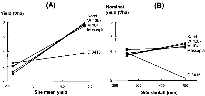
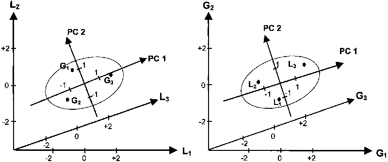
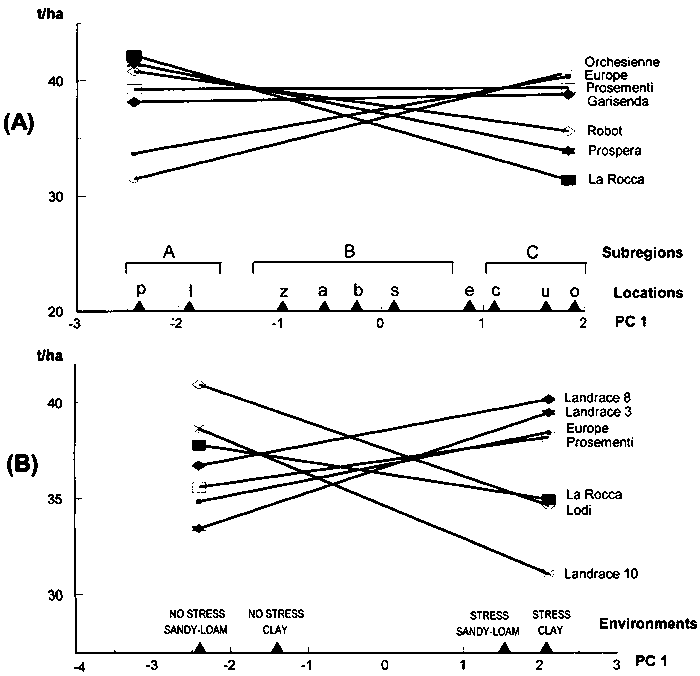
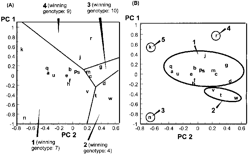
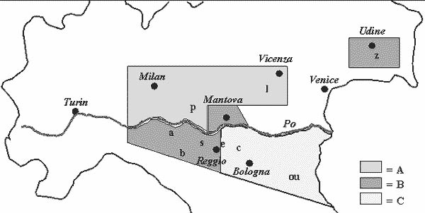
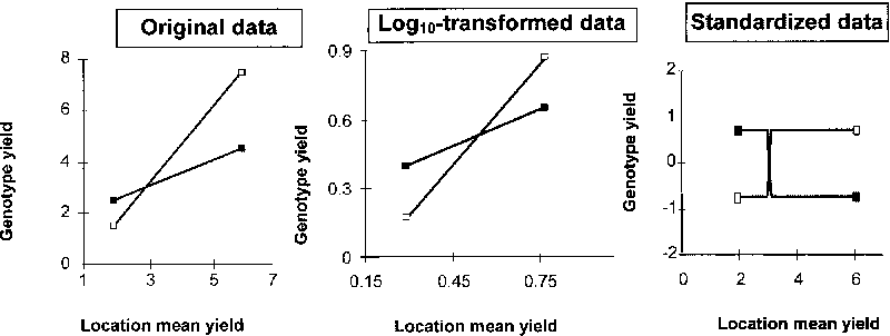
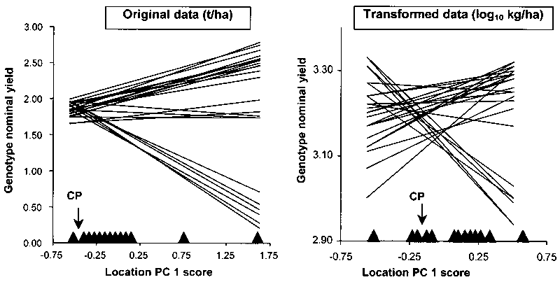