14. Calculation with grids using GIS

14.1. Map calculations

In a grid, each pixel has a characteristic attached to it. This can be a code but also a number, as for example water level or topographic level. Once grids are compared in the same location, it becomes straightforward that you can make calculations between grids.

Let us look at an example. In Figure 14.1 a cross-section is presented from the floodplains in Pais Pesca with the brown line representing the topography of the land and the blue line the water level.

FIGURE 14.1
Cross-section of the floodplain of Pais Pesca

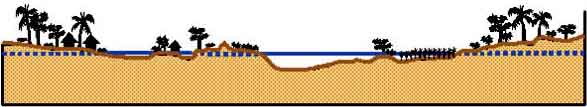
In the cross-section, the blue line is a surface plot generated for water levels (like the one you made before) and you see immediately that there is water in places where the topo-level (brown line) is lower than the surface plot. To make a flood map, i.e. the real extent of flooding, you need the generated water level grid and a grid representing the topography of the floodplains.

Both grid files have values attached to each pixel. This allows us to calculate the water depth at each location presented by a pixel by simply subtracting the value of the topo-level from the water level.

Water depth = Water level-Topo level

An example of this calculation is presented in Table 14.1, and it is clear that once the value of the water depth becomes negative the area is dry.

TABLE 14.1
Example of calculation of water depth in the floodplain of Pais Pesca

The same procedure, but now in ArcView:

1. Start ArcView, open a New Project, and a New View. Add the Themes ‘Pais_Pesca_country.shp’, ‘Flood_districts.shp’, ‘Flood_district_topo.shp’, and ‘Flood_levels.shp’ from the ‘12_Calc_with_grids’ folder. Project the view (via the menu bar: View/Properties.../Projection..., ‘Equal area cylindrical’), and set the distance units to meters.

2. Make first a topographic map of the floodplain districts involved: First you want to make a grid of the ‘Flood districts.shp’ Theme (Theme/Convert to Grid..., Grid name: ‘Mask’, Output Grid extend Same as View, Cellsize 100 meters), set this grid as a mask in the analysis properties, and only after that interpolate the topolevels.

3. Make the ‘Flood_district_topo.shp’ Theme active, go via the menu bar to Surface/Interpolate Grid... (output grid extend: Same as View, Cell size 100 meters, Method: IDW, Z-value field: what do you think?^[16]). This interpolation may take a long time. Save the grid as ‘Floodtopo’ in a folder you choose. After the interpolation, you can load the legend that was made for this grid (‘Topo.avl’). If you do not remember how to load a legend, please have a look at the tip on page 53.

FIGURE 14.2
The topographic level of the districts involved

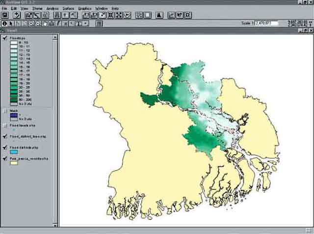
If the interpolation takes too long, you can stop the process and load the interpolated grid. (From the folder ‘12_Calc_with_grids’, Data Source Type: Grid Data Source, ‘floodtopo’. If you can not add the grid to your View, and you are sure the grid is in a certain subfolder, check if the path to this subfolder follows the naming convention of ArcView (see the remarks on the naming convention on page 52, it might be that somewhere in the path to your file there is a space, or a name that is longer than 13 characters. After you added the grid, load the legend [in the legend editor]: ‘topo.avl’). The results of your efforts should look like Figure 14.2.

The previous interpolation took such a long time, because ArcView had to calculate the waterlevel for every cell in the view (3 767 cells by 3 983 cells, resulting in a total of 15 003 961 cells!). The calculation time can be reduced, when you reduce the number of cells that need to be calculated. You can do this by increasing the cell size. If you increase the cell size from 100 to 1 000, the number of cells decreases to (377 * 398) = 150 046 cells. By doing so, the grid you create will have quite a low resolution, with which it is difficult to do meaningful analysis. Another way to reduce the number of cells to be calculated, and keep the same resolution (CellSize: 100), is to zoom in on the area where you want the calculation to take place, and make the Output Grid Extent ‘Same As Display’. If you do this, you have to pay special attention that you include the whole area you want the calculation with, otherwise your calculation is worthless, and you have to do it again.

Now you need to make a grid with the water levels during October. Have a look at the table of attributes of the Theme ‘Flood_levels.shp’. You will see that there are two water levels per record, October and June water level, for now you will make the grid with the October water level.

4. Make sure you still have the mask set (in the menu bar: Analysis/Properties...) (this should be ‘Mask’, the grid you made previously at 3. of ‘flood_district_topo.shp’). Activate the ‘Flood_levels.shp’ Theme. Go via the menu bar to Surface/Interpolate Grid... (Output Grid Extend: Same as View [if the previous interpolation took a long time you can reduce that this time by zooming in on ‘Flood_levels.shp’ and making the Output Grid Extend: Same As Display], Cell size 100 meters, Method: IDW, Z-value field: what do you think?^[17]). Also this might take a long time, and also for this interpolation the result is already in the folder if you can not wait for the interpolation to take place (‘Watersurf’, legend: ‘Water_levels.avl’).

If you have interpolated the grid yourself, you can save this grid as ‘Watersurf’ (menu bar: Theme/Save Data Set...) in a folder you choose, and change the name of this Theme into Watersurf (Theme/Properties...). Only if you change the name of the Theme (via the menu bar: Theme/Properties..., Theme Name:) will the this name appear in the Table of content (on the left side of the View).

Why do you not see a water level in the river and big lake in the centre of the flood districts?^[18]

Now you have the two grids ‘Watersurf’ and ‘Floodtopo’ of the same area in your View, both with the same grid dimensions of 100 meters. Calculate the water depth in the floodplain with the formula: Water depth = Water level - Topo level.

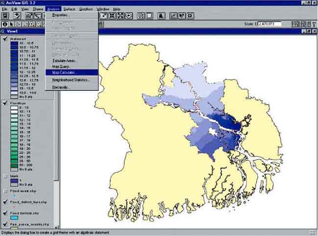
1. Go to Analysis/Map Calculator... via the menu bar (Figure 14.3). The Map Calculation window opens (Figure 14.4).

FIGURE 14.3
Opening the map calculation menu

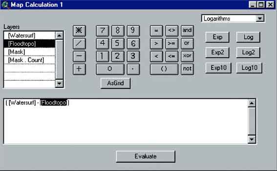
FIGURE 14.4
Calculating the water depth in the floodplain

2. In the window you see the names of the grids; [Watersurf], [Floodtopo], [Mask] and [Mask.count]. The calculation you need to carry out will be with the first two. Simply enter the formula by double-clicking [Watersurf], then ‘-’, followed by double-clicking [Floodtopo]. Click on Evaluate to start the calculation, and close the Map Calculation window after the results appear as the Theme ‘Map calculation 1’. Save this Theme^[19] as ‘Fldepth’, before you change anything else!!! (Theme/Save Data Set...).

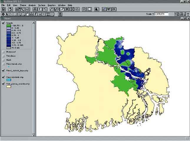
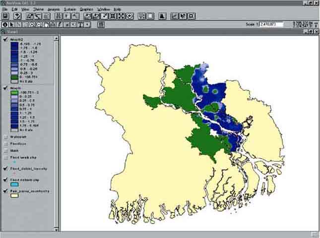
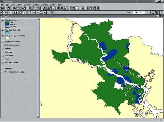
3. Redo the legend of ‘Fldepth’ in such a way that water becomes various gradients of blue and dry land becomes one grade of green (Figure 14.5). You will see that the latter is not easy, as you have to think in negative values. It is easier to change the calculation to Water depth = Floodtopo - Watersurf. Do the calculation again, but now first [Floodtopo]. Positive values signify dry land, while negative values become water depth (Figure 14.6). Save this Theme as ‘fldepth2’.

FIGURE 14.5
Floodmap of Pais Pesca

FIGURE 14.6
Floodmap of Pais Pesca, reversed calculation

4. You can save the project as: ‘Pais Pesca floodmap.apr’ in a folder you choose.

Note:

During calculation or grid manipulation you can get the following message:

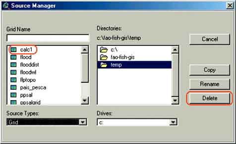
This means that you have deleted grid files from the working directory. NEVER DO THIS! Always use Manage Data Sources in the File menu (via File/Manage Data Sources... in the menu bar, Figure 14.7). If you select this, the Source Manager window will popup (Figure 14.8) and here you can copy, move or delete grids.

FIGURE 14.7
Starting the Data Source Manager

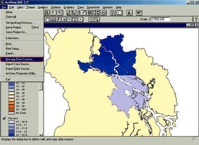
FIGURE 14.8
The Source Manager

14.2. Reclassifying

The calculation of the water depth gives a large number of different water depths in the floodplain of Pais Pesca. However, in some calculations we are not interested in the water depth but only whether a certain area is flooded or not. Working with all the different water levels makes further calculations unnecessarily cumbersome. An easy way to overcome this problem is to reclassify the data, i.e. you give a specific value to all pixels representing a dry (0) area and another specific value (1) to all pixels that are flooded.

1. Continue where you stopped with the previous exercise, or open the project you saved: ‘Pais Pesca Floodmap.apr’.

2. Activate the Theme ‘Fldepth’.

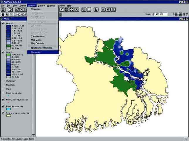
3. Go to Analysis/Reclassify... via the menu bar (Figure 14.9); the Reclassify Values window will pop up. For the classification into dry and flooded we obviously only need two classes (dry and flooded).

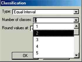
4. Click on Classify... and select 2 classes in the Classification window (Figure 14.10) and click OK.

5. The Reclassify Values window appears again, now with two classes. All negative values that we calculated are dry areas, so you use the values -200 to 0 for dry land and the values 0 to 200 for flooded land. Click OK and the new Map will appear (Figure 14.11).

FIGURE 14.9
Opening the reclassify window

FIGURE 14.10
Selecting two classes to reclassify

6. Give the file a new name, arrange the legend (by double clicking the theme, or by going to Theme/Edit Legend...via the menu bar). If you have forgotten how to arrange a Legend, please have a look at Graphical displays in the Map View, on page 15.

7. Make yourself a flood map of June (Figure 14.12), and save the project again.

FIGURE 14.11
The new floodmap of Pais Pesca of October

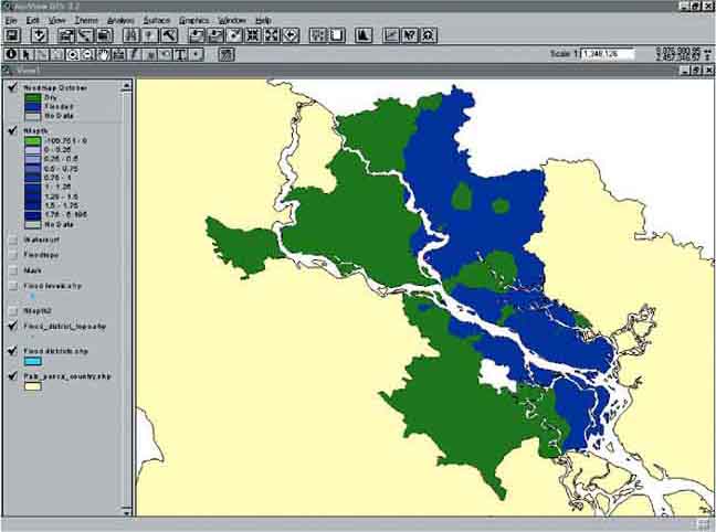
FIGURE 14.12
Floodmap of June

14.3. Querying

In a query, you try to find locations or areas on a map that fulfils certain criteria. This can be done with two criteria using two GIS Themes but it can also be a more complicated query using a large number of Themes.

Some examples:

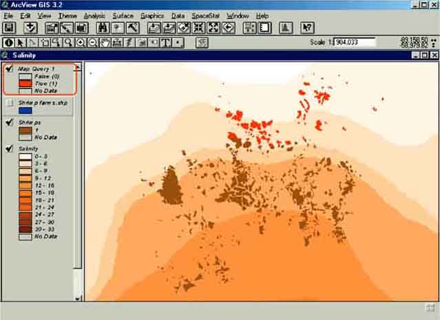
• Find all the areas with a salinity level of 15 ppt and shrimp farming as a major crop. For this two GIS themes are needed, i.e. Salinity and shrimp farms.

• Find all the areas with alluvial soils, medium rainfall and rice as major crop. Here three themes are needed, i.e. soil map, rainfall map and land use map.

• Find all the villages with more than 50 percent fishers, more then 50 percent of Hindu house holds, average income of these households less then 150 $/year and fishing in the river. Four GIS themes are needed for this query, i.e. Occupation, Income, Religion, and Catching area.

14.3.1. Shrimp farming in the coastal areas of Pais Pesca

In the coastal provinces of Pais Pesca shrimp farming expanded rapidly from 8 000 ha in 1992 to 86 000 ha in 2001. The applied system^[20] is extensive with low stocking densities of post larvae, mostly obtained from the wild. The system is an alternation of rice with shrimps, with rainfed rice during the wet season and one crop of shrimps during the dry season. Average yields of shrimps are in the order of 200-400 kg/ha/crop. However the expansion of shrimp farming was unplanned and three major problems developed over time:

• In the mid 1990s the first large problems with Monodon baculo virus (MBV) arrived followed by a serious outbreak of White Spot disease in 1998, which almost completely wiped out the shrimp production.

• Further due to the expansion and intensification of shrimp farming a serious conflict developed between the large shrimp farmers and the paddy farmers. This occurred as the shrimp farmers tried to grow two crops and consequently shrimp farming extended into the wet season resulting in a salt intrusion seriously hampering the cultivation of rice in the same area.

• Shrimp farming encroached into the mangrove forest, the major biosphere reserve of Pais Pesca. Shrimp ponds were constructed in acid sulphate soils in the mangrove area resulting in serious acidification of the surface water at the beginning of the rainy season.

In 2000 the Department of Fisheries carried out an extensive survey in the coastal area and collected the following information:

• Location and size of the shrimp farms;

• Average yields;

• Water quality;

• Disease occurrence.

You will make an analysis in GIS to demonstrate how grids and querying of different grids can be used to support management options for shrimp farming in Pais Pesca.

Shrimp farming analysis

The Ministry of Agriculture recommended reducing the number of shrimp farms in the agriculture zones of the coastal belt, i.e. the areas with low surface water salinities (5 ppt) in the dry season where paddy can be transplanted early in the rainy season. Therefore it requested the Department of Fisheries to give an indication of the consequences of this strategy.

1. Open ArcView, New Project, New View.

2. Set the working directory to a directory of your choice (for instance: C:\FAO_GIS\Temp), the projection of the View to ‘Equal-Area Cylindrical’, and the Distance and Map Units to meters.

3. Add the following Themes from the ‘13_Querying_shrimp’ folder to the View: ‘Pais Pesca country.shp’, ‘Shrimpfarms.shp’, ‘shrimp yields.shp’ (all being Feature data sources), and the Grid data source ‘Salgrid’. The folder contains also a legend for the salinity grid (‘Salgrid’) for use if you want to.

Salgrid is the same grid as you have made in the exercise on page 58. ‘Shrimpfarms.shp’ is a polygon file of all the shrimp farms in the coastal area of Pais Pesca. ‘Shrimp yield.shp’ a point file of the location of each farm, its average yields, and other data. ‘Pais pesca country.shp’ is a polygon file containing the outline of the country.

4. First you want to know how many shrimp ponds are located in the low salinity area. You can do this with a query between two grids. So first you have to convert the ‘Shrimpfarms.shp’ to a grid. You want to work in hectares so you choose a grid output CellSize of 100 m (resulting in an area of 100 m by 100 m = 1 hectare). Use the ‘Id’ field for cell values, and do not forget to rename the grid to ‘shrimps’. To prevent this calculation to take too much time you might want to zoom in on the shrimp farms, and do the interpolation with the Output Grid Extent: Same As Display.

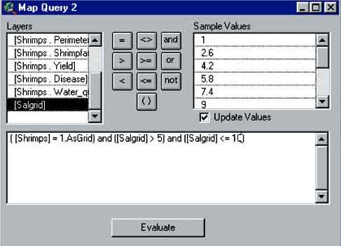
You need to query this shrimp grid with the salinity grid and use as selection criteria: shrimp ponds = true, ([Shrimps] = 1.AsGrid) and salinity <= 5 ([Salgrid] <= 5). In other words: of all the spots in the shrimp Theme where there is a farm present (or equal to the desired value of the pixels, in this case 1, as there is no other value), find the spots where the salinity (on the salgrid Theme) is equal or lower than 5 ppt.

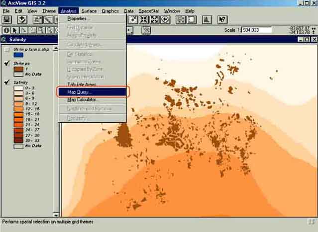
5. Go to Analysis/Map Query... via the menu bar (Figure 14.13).

FIGURE 14.13
Opening Map Query

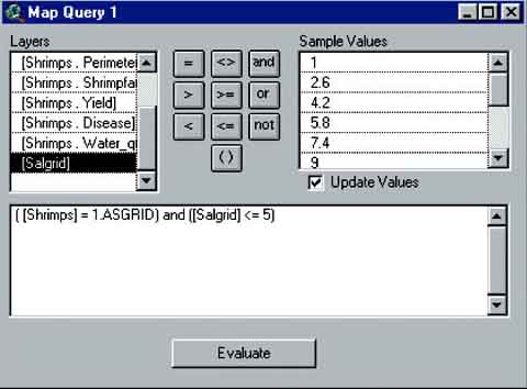
6. The Map Query window will pop up and you need to put the selection criteria in the window: ([Shrimps] = 1.AsGrid) and ([Salgrid] <= 5). You can do this in several ways: You can type this sentence in the lower window, or you can select the arguments from the top part of the Map Query window; First you double click on [Shrimps], then you click on ‘=‘, and then you click on ‘1’. When you have clicked on ‘1’ you see in the query line appear: ‘1.AsGrid’. This is normal, but you can also use a number you put in yourself (like ‘1’) which will also work. Then click on ‘and’ in the middle of the Map Query window, after which you double click on [Salgrid], ‘<=‘, and type ‘5’. You can not select ‘5’ from the values part, so you have to type this value. (Figure 14.14). Click on Evaluate.

FIGURE 14.14
Selecting the criteria for the query

FIGURE 14.15
Results of Querying shrimp farms and salinity

7. The query will run and after some time the results of the query, which is called ‘Map Query 1’ will appear in the View (Figure 14.15). First close the Map Query 1 window, and then do not forget to save this query as ‘SHRSAL5’^[21] (Theme/Save Dataset...). If you open the Theme attribute table of the grid you will see that there are approximately 14 800 pixels of shrimp pond, meaning that 14 800 ha of shrimp ponds are located in the low salinity zone. We converted the original shapefile to a grid with a cell size of 100 metres by 100 metres, which is 1 hectare. If the number differs greatly from 14 800 you need to check the projection of the view, to make sure it is Equal Area Cylindrical.

8. To get a more clear picture you also want to know how many farms are located in the other zones and we make the query Shrimp farms yes and 5> salinity<=10.In other words, find the shrimp farms which are located in areas where the salinity is higher than 5 ppt and lower or equal to 10 ppt (Figure 14.16).

FIGURE 14.16
Querying with two grids and three criteria

9. Fill in Table 14.2:

TABLE 14.2
Salinity and number of shrimp farms

You see that more then 50 percent of the farms are located in the salinity zone of 5-10 ppt. But still approximately 15 000 ha are located in the low salinity zone and the question is if you can get more information on the status of the farming system in this area before you decide to close them. For this you have to look at the yields of the farms. The location and the yields of the individual farms are available in the ‘Shrimp yields.shp’ Theme. This is a point shapefile so you can use it to generate a grid for the yields.

10. Make a surface grid of the yields (through interpolation, menu bar: Surface/Interpolate Grid...), Output grid size 100 metres, with the Shrimps grid set as mask. Remember that this might take a while! (To reduce the time, zoom in on the ‘Shrimp yield.shp’ Theme, and make the Output Grid Extent: Same As Display). After the interpolation is completed you can load a legend for this grid named ‘shrimp_yield_grid.avl’ (in the 13_Querying_shrimp folder).

If you do it correctly you will get a grid like the one presented in Figure 14.17.

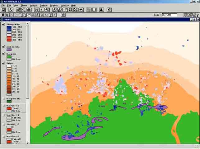
FIGURE 14.17
Shrimp farming yield in the different salinity zones of Pais Pesca

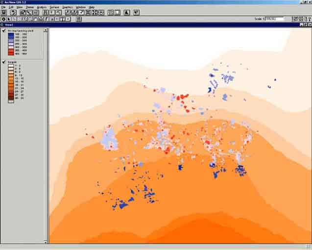
The results change the picture somewhat. We see yields (blue) of about 150-250 kg/ha/crop in the northeast in the salinity zone of 0-3 ppt. In the zones of 3-12 ppt yields are in the order of 250-450 kg/ha/crop (light blue to red) and in the south you suddenly observe very low yields (dark blue) of 100-150 kg/ha/crop in salinities from 12-15 ppt.

A first conclusion could be to recommend to the Ministry of Agriculture to close the shrimp farms in the salinity zones of 0-3 ppt. Query again how many hectares of shrimp farms would be closed under this option^[22]. Secondly you found another problem in the 12-15 ppt zone. The salinity levels are favourable for culture of P. monodon, so there must be another factor causing these very low yields in the southern part.

In the Theme table of the ‘Shrimp farms’ shapefile we have data on Shrimp diseases and water quality. With simple queries of this theme table you can select the farms with a ‘high disease’ occurrence, a ‘low disease’ occurrence, ‘bad water quality’, ‘reasonable water quality’, etc. Try this out (Remember: First you have to convert the Theme ‘shrimpfarms.shp’ into a grid (menu bar: Theme/Convert to Grid...), with a cell size of 100 metres, while picking the relevant Conversion Field, before you can query it in the Map Query).

You will find that the low production in the south is related to ‘high disease occurrence’ and ‘bad water quality’. The question now is what is the cause of this problem.

Add the Theme ‘Mangrove.shp’. You can see that the farms with the low productions are mainly located in the mangrove belt.

How many hectares of shrimp farm are located in the mangrove belt?

1. Convert the ‘Mangrove.shp’ Theme to a grid, with grid size 100 meters (Check your working directory and projection, zoom in on the Theme, and make the conversion Output Grid Extent: Same As Display).

2. Query the Mangrove grid with the Shrimp farm grid (Figure 14.18), which will give you Figure 14.19.

FIGURE 14.18
Querying the mangrove grid with the shrimp farm grid

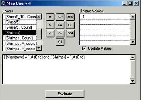
FIGURE 14.19
Shrimp farms in the mangrove forest of Pais Pesca

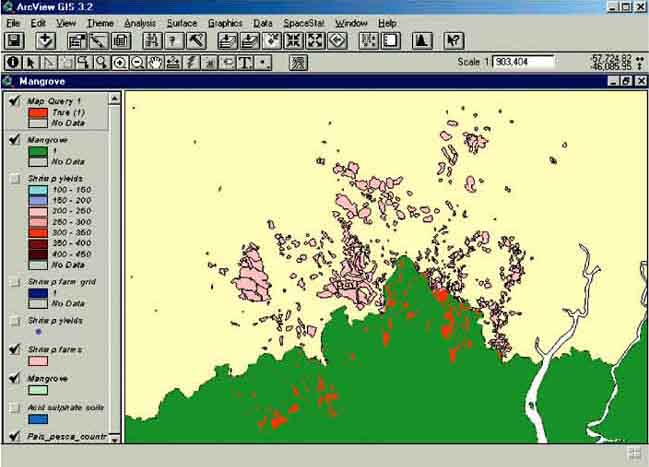
From the Theme table of the Map Query Theme you see that approximately 15 589 pixels are selected with this query, meaning that 15 589 ha of shrimp ponds are constructed in the mangrove belt of Pais Pesca (as one cell is 100 metres by 100 metres). Query further the Mangrove grid with the surface grid of the yields, after which you will get the following distribution (Table 14.3):

TABLE 14.3
Area of shrimp ponds according to average yields in the mangrove belt of Pais Pesca

From this distribution we see that 8334 ha has low annual yields of 100-200 kg/ha/crop, this apart from the favourable salinity of this area. There must be a negative factor affecting the production (again, if your numbers are not the same as given in the table, check your projection, to see whether you use Equal-Area Cylindrical).

The major reason for the low productions, high disease rate, and bad water quality might be that ponds are constructed on acid sulphate soils. These soils are a normal phenomena in mangrove forests. No problems will arise if they are left undisturbed. However, disturbing them (by for instance digging ponds into these layers, or ploughing) results in leaching of sulphuric acid and a reduced pH of the surface waters(de Graaf et al., 1998).

Add the ‘Acid_soil.shp’ Theme and this relation becomes clear (Figure 14.20). How many hectares of shrimp farms are constructed on acid sulphate soils? What would be your recommendation regarding the shrimp ponds in the low salinity areas and in the mangrove belt? Try to answer these questions by querying (do not forget to convert the ‘Acid_soil.shp’ Theme first).

FIGURE 14.20
Shrimp ponds, mangrove and acid sulphate soils in Pais Pesca

14.3.2. Protection of fish stocks and the creation of protected areas in Lake Kadim, Pais Pesca

Lake Kadim is the largest fresh water lake of Pais Pesca (220 km²). Fisheries at the lake is highly productive with an annual catch of about 2 000 metric tonnes/year and it provides an income to 1 300 professional fishers. There are two major fish species:

• Carpio felixiensis. A phytoplankton feeder, mainly living in water depth up till 10 metres, annual catch 900 metric tonnes.

• Clupea pepeiensis a pelagic, zooplanktivore, annual catches 700 metric tonnes.

The fishers demanded the creation of protected areas, where fishing is closed during the spawning season for protection of the stocks. However, they could not agree where to create the sanctuaries and asked the Department of Fisheries (DoF) for assistance. In 1999, an extensive survey has been carried out during the spawning season by DoF, to provide scientific data for selection of spawning sanctuaries. Systematic sampling was carried out all over the lake and the following data was collected:

• Water depth (m);

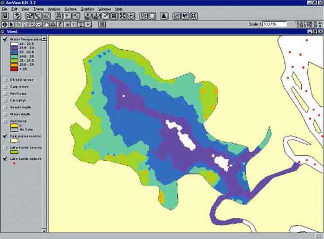
• Water temperature (°C);

• Secchi depth (m);

• Chlorophyll A(m g/l);

• Larval abundance clupeids (number/m²);

• Larval abundance of carp(number/m²);

• Abundance of adult carp (number/m²).

Analysis of the data in GIS will support the decision where to create fish spawning sanctuaries as it lets you understand the basic mechanisms behind spawning and spatial distribution of the adult fish and their larvae and eggs.

1. Open ArcView, New Project, New View.

2. Add the Themes ‘Lake kadim data.shp’(containing all data and georeferences concerning the different sampling sites in Lake Kadim), ‘Lake kadim boundary.shp’, and ‘pais pesca country.shp’ from the ‘14_Lake_Kadim’ folder.

3. Check the working directory and set the projection.

4. As you are going to work at Lake Kadim only, you will first need to make a grid of the ‘Lake Kadim boundary’ shapefile, output grid size 100 metres, so each pixel equals 1 hectare. Save this grid as ‘kadimbnd’.

5. Set this grid as mask.

6. Activate ‘lake Kadim data’ and make a surface grid^[23] (by interpolating) of the ‘water depth’ with ‘IDW’ and a 100 metres grid cell size. If you do this interpolation on the View it will take a long time, so Zoom in on Lake Kadim, and make the Output Grid Extent: Same As Display. Save the new grid as ‘Kaddepth’.

7. Make similar surface grids for ‘secchi depth’, ‘chlorophyll’, ‘adult carp abundance’, ‘carp larvae abundance’, ‘clupeids larvae abundance’ and ‘water temperature’.

The different grids are presented below, (Figure 14.21 until Figure 14.27). The first impressions are:

• The deeper parts are in the middle of the lake.

• Low Secchi disc, high chlorophyll concentration, high carp larvae density, high adult carp density and higher surface water temperatures are in the northwest of the lake.

• While the highest density of clupeid larvae is in the centre of the lake.

FIGURE 14.21
Water depth of Lake Kadim

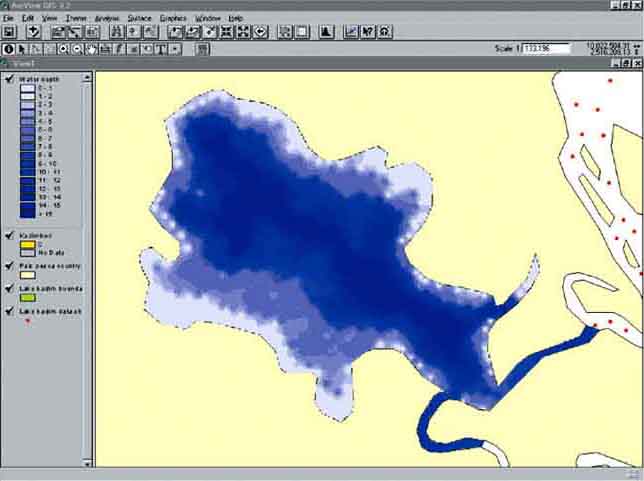
FIGURE 14.22
Secchi depth of Lake Kadim

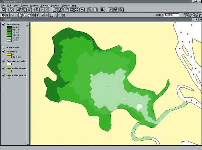
FIGURE 14.23
Chlorophyll concentration in Lake Kadim

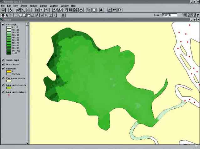
FIGURE 14.24
Carp larvae density in Lake Kadim

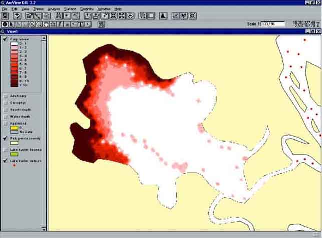
FIGURE 14.25
Clupeid larvae density in Lake Kadim

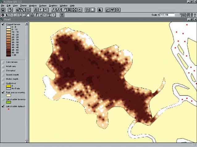
FIGURE 14.26
Adult carp density in Lake Kadim

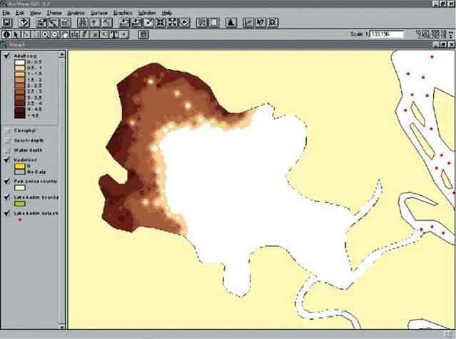
FIGURE 14.27
Water temperatures in Lake Kadim

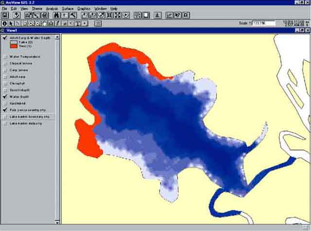
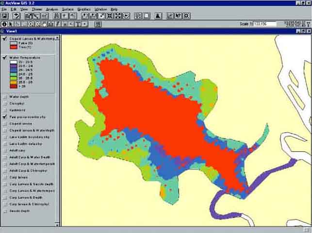
However, these are only impressions. Check if an analysis in GIS can confirm the following hypothesis: Adult carp are mainly found in the shallow waters. For this you need to query the water depth grid with the adult carp grid (Figure 14.28). The results (Figure 14.29) show that there are adult carp in shallow water, but only in the northwestern part of the lake. In the shallow waters in the southeast, the densities of adult carp are low.

FIGURE 14.28
The query between water depth and adult carps

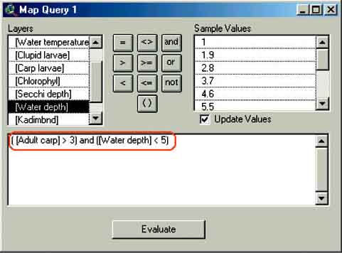
FIGURE 14.29
The results of the query between water depth and adult carps

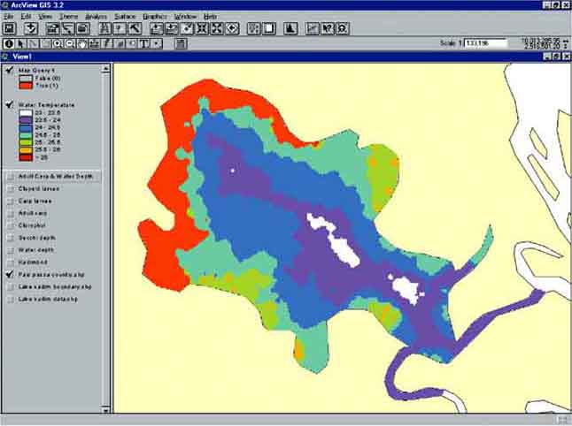
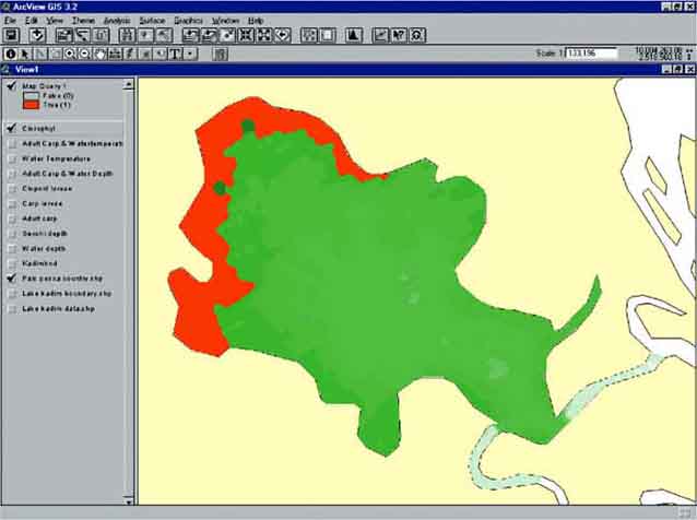
Maybe adult carp prefer higher water temperatures. Therefore, query the adult carp grid with the water temperature grid (Figure 14.30). The results are presented in Figure 14.31.

FIGURE 14.30
The query between adult carps and water temperature

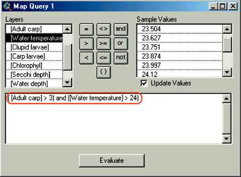
FIGURE 14.31
The results of the query between adult carps and water temperature

The carp is phytophageous so it could be that the abundance of phytoplankton is a factor in the distribution of the adult carp. Therefore, query the chlorophyll grid with the adult carp grid (Figure 14.32). The results are presented in Figure 14.33. Indeed you see a very good match between the chlorophyll and the adult carp distribution which could mean that chlorophyll or the abundance of phytoplankton is a major factor for the distribution of adult carp.

FIGURE 14.32
The query between adult carps and chlorophyll

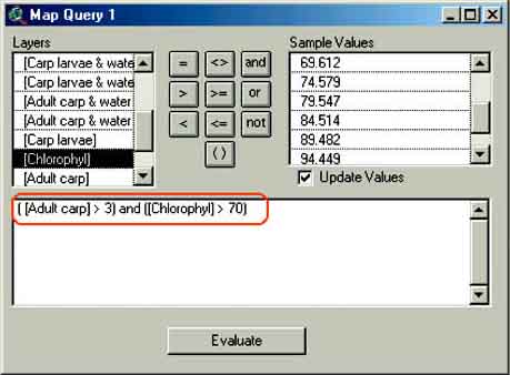
FIGURE 14.33
The results of the query between adult carps and chlorophyll

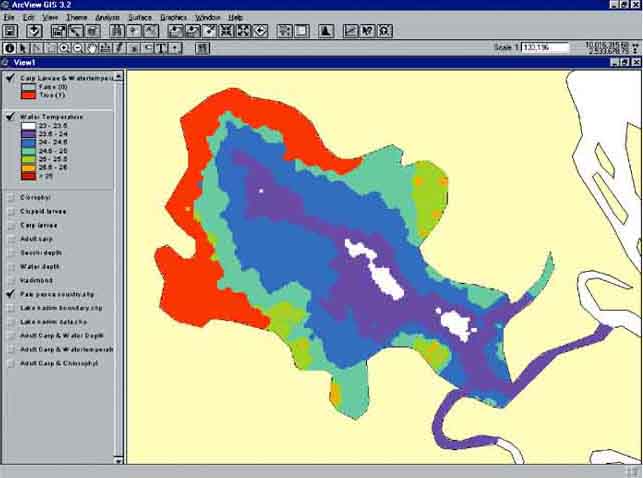
What about the distribution of carp larvae, would that be related to water temperature? Query the carp larvae grid with the temperature grid (Figure 14.34). The results are presented in Figure 14.35.

FIGURE 14.34
The query between carp larvae and temperature

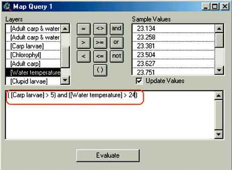
FIGURE 14.35
The results of the query between carp larvae and temperature

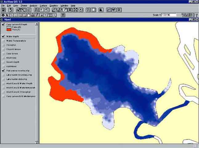
What about the water depth and the distribution of carp larvae? (Figure 14.36). The result of the query between the water depth and the abundance of carp larvae is presented in Figure 14.37. Again, you see shallow parts where there are no carp larvae, especially the northeastern and southern shorelines.

FIGURE 14.36
The query between carp larvae and water depth

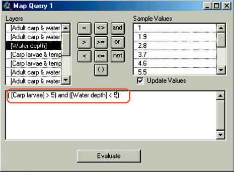
FIGURE 14.37
The results of the query between carp larvae and water depth

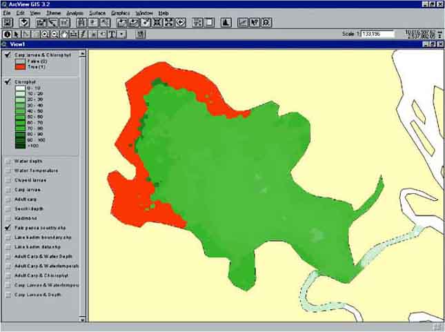
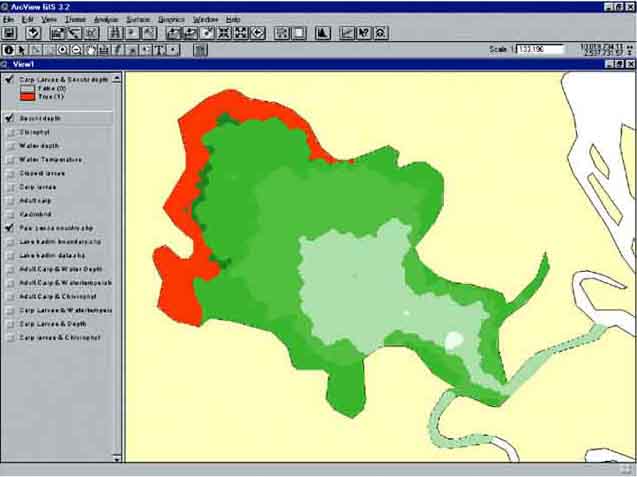
Query the carp larvae grid with the chlorophyll grid (Figure 14.38). The results are presented in Figure 14.39. What are your conclusions?

FIGURE 14.38
The query between carp larvae and chlorophyll concentration

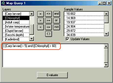
FIGURE 14.39
The result of the query between carp larvae and chlorophyll concentration

Query the carp larvae grid with the secchi depth grid (Figure 14.40). The results are presented in Figure 14.41. What are your conclusions?

FIGURE 14.40
The query between carp larvae and Secchi disk depth

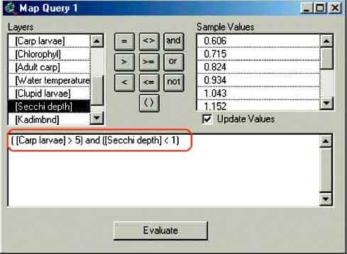
FIGURE 14.41
The result of the query between carp larvae and Secchi disk depth

A first look at the distribution pattern of the Clupeid larvae indicates immediately that this is not related to chlorophyll or secchi depth. However, it could be related to water depth or surface water temperature as the highest densities are found in the middle of Lake Kadim.

Query the ‘clupeid larvae’ grid with the ‘water depth’ grid (Figure 14.42). The results are presented in Figure 14.43. The created grid is reasonable but there are still high densities of clupeid larvae outside the created grid. Make the grid again but now with a water depth of 6 metres or more. Does this improve the situation?

FIGURE 14.42
The query between clupeid larvae and water depth

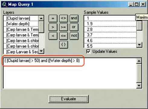
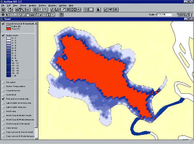
FIGURE 14.43
The results of the query between clupeid larvae and water depth

Query the Clupeid larvae grid with the water temperature grid (Figure 14.44). The results are presented in Figure 14.45. The created grid matches better then the water depth especially at spot points and it seems that water temperature, especially in the central part is an important factor for the distribution of clupeid larvae.

FIGURE 14.44
The query between clupeid larvae and water temperature

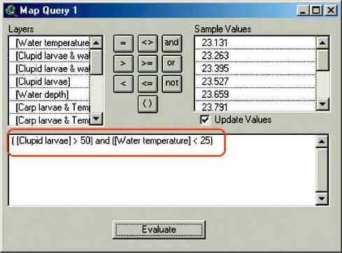
FIGURE 14.45
The result of the query between clupeid larvae and water temperature

Conclusions

• Adult Carpio felixiensis mainly concentrates in the shallow waters located in the northwestern part of Lake Kadim. The major driving force behind this mechanism is most likely feeding as its distribution follows the distribution pattern of chlorophyll. The newly born larvae of Carpio felixiensis follow the same distribution pattern.

• The larvae of Clupea pepeiensis have a completely different distribution as they aggregate in the deeper waters. In the deeper waters this distribution is most likely related to water temperature.

It should however be realized that the relations made visible through querying of grids is a kind of visualisation only. Direct relations between adult carp densities and chlorophyll or clupeid larvae and water temperature are not quantified or statistically verified. This can only be done through regression analysis and this will be discussed in the next chapter.

For the establishment of a fish sanctuary these findings have complications as closing fisheries in the northeastern shallow and eutrophic waters will certainly protect the carp stocks but this will not protect the clupeid stocks. Only a complete closure of fisheries for several months will protect both stocks.