6. CHANGES IN THE FISH COMMUNITY OF LAKE MWERU IN RELATION WITH EFFORT AND WATER LEVEL

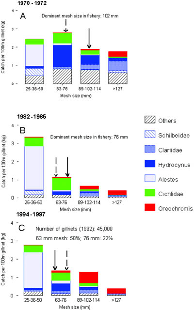
By comparing catch rates in experimental surveys with fleets of gillnets with a range of mesh sizes conducted over three periods between 1970 and 1999 in the lake, changes by species and on a fish community level can be observed^[9]. The indicators we will use are changes in species composition of the experimental catch, changes in size and catch rate by species and changes in the size-structures of the fish community based on biomass-size distributions. By relating these changes to fluctuations in lake level and to what is known about effort development in the fishery we can deduce the effects changing and increasing fishing effort would have on the fish community of lake Mweru. Over the period from 1970 to 1999 examined here, effort on the lake has been and still is dominated by gillnets. Mesh sizes used in the fishery have decreased from 76 to 102 mm in the 1970s, via 63-76 mm in the 1980s to mainly 63 mm in the 1990s (Zwieten and Kapasa, 1995, 1996; Goudswaard, 1999).

Gillnets only last for a few years and a whole fishery can shift rapidly from one dominant mesh size to another in response to changes in size structure and biomass of the commercially important species in a fish community. Catch rates in the fishery have dropped from 10 to 12 kg per standardized net before 1964 to around 4 to 5 kg from 1967 onwards (Figure 9), decreasing further since to about one to two kilos now. The vast drop over three years after 1964 coincided with a massive increase in effort both through an increase in synthetic gillnets that became accessible to fishers after independence, an increase in number of fishers and a drop in water levels during a dry spell lasting five years. Increases and drops in catch rates of the fleet of experimental gillnets - i.e. with a range of mesh sizes between 25 and 178 mm stretched mesh other than in the fishery where only a few mesh sizes are used - are generally lower than catch rates from the fishery^[10]. They do not appear to follow variations in water levels closely (Figure 8). Changes in aggregated catches and catch rates do not reveal the underlying changes in species composition targeted by the fishery, while total number of species caught in the experimental surveys did not change between the three decades as well: 46 in the 1970s, via 38 to 48 in the 1990s. However, Shannon’s diversity index (H’), which includes information on relative abundance, indicated that a change in diversity had taken place over the 30 year period examined. The index decreased from 2.37 ± 0.07 (mean and confidence interval) via 1.21 ± 0.12 to 1.49 ± 0.14 in the three periods examined from 1970 to 1996. Thus in experimental catches the number of species did not change, whereas the relative abundance of species did.

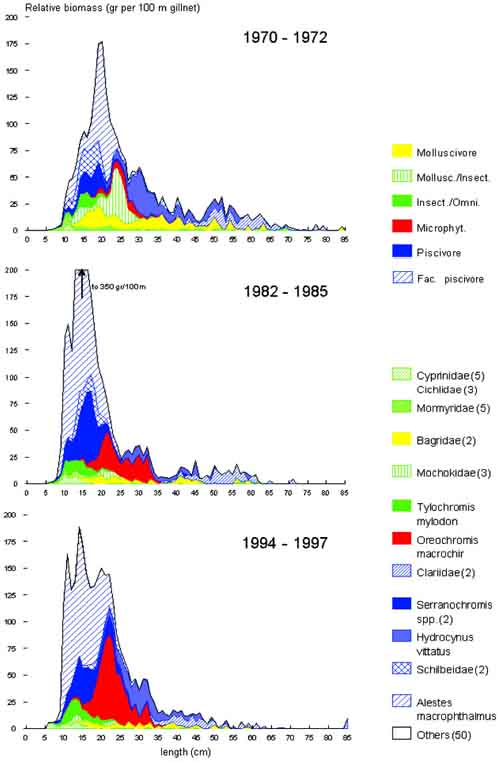
These changes are reflected both on a species and on community level. We will discuss these first before trying to relate them to effects of changes in effort and productivity. The biomass-size distributions over the three periods in subsequent decades (Figure 10) contain in a highly aggregated form a wealth of information. The aggregations are over:

time: three years per decade;

space: nine sampling sites distributed over the whole lake,

and category: twelve species and species groups aggregated over catches of in total 78 species, that are simultaneously represented as broadly defined trophic groups as well.

The following can be noted immediately from the graphs:

1. A decreased contribution to the total biomass of large sized individuals of different species from the 1970s to the 1990s, in particular the larger bagrid and clariid catfishes and large Mormyridae, and the large piscivore Hydrocynus vittatus.

2. An enormous variability in biomass of the small sized species and specimens, in particular Alestes macrophthalmus,

3. A shift in importance of species: an increase in biomass and size of the cichlids Serranochromis macrocephalus (dark blue), of Tylochromis mylodon (green), and in particular of Oreochromis mweruensis (red) and decreased contribution of Mochokidae and Schilbeidae.

6.1 Changes on a species level

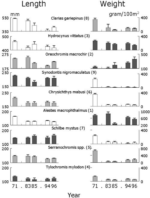
Changes in the mean length and mean weight in the catch of the nine most important species in the in the fishery (Figure 11) reveal that:

1. All species decreased in average length comparing the two years 1971 and 1996, except Schilbe mystus, but with no consistent pattern over all species at intermediate years. Species that obtain larger sizes, decreased >20 percent in average length. This includes Alestes macrophthalmus that can grow up to 50 cm, but has a low mean size because of high abundance of small individuals. Similarly large Mormyridae, other large Clariidae and the bagrid Auchenoglanis occidentalis (not shown) have decreased in average length by similar proportions. Of the remaining species shown in Figure 11, a few exhibited a consistent decrease in length over time. But in almost all cases including that of the piscivore Hydrocynus, variability in mean length between years was either high, did not change significantly after an initial drop, or even increased again. In particular the cichlid species Tylochromis and Serranochromis, targets of most of the fisheries, did not change much and in case of Oreochromis mean length even increased again between 1994 and 1996.

2. All species declined in mean weight in the catch, except Oreochromis mweruensis for which the mean weight in the catch increased consistently over the period examined! The mean weight of the other two cichlids fluctuated (Tylochromis) or increased (Serranochromis) since the initial drop of between 50 and 80 percent. The mean weight in the catch of the two piscivores Hydrocynus and Alestes, fluctuated greatly. That of the other species consistently decreased from 1971 onwards.

FIGURE 10. Biomass-size distributions of Lake Mweru over three periods. Stacked areas in the graph indicate species (groups), colours indicate broad trophic categories. Biomass is expressed as standardized average catch per unit of effort of 100 m2 of gillnet by 1 cm length class in the catch over the periods indicated and over all sites sampled during that period. Catch rates were corrected for net selectivity and amount of effort per sampling site. In brackets are the numbers of species combined in that particular group. See text for further explanation.

Apart from species that grow to large sizes, there is no consistent unidirectional pattern in both indicators mean length and mean weight as would be predicted from the unidirectional increase in fishing pressure after 1971 (e.g. Welcomme, 1999). Large individuals of some species have been hit hard, but with differing results with regard to their biomass. Mean lengths of smaller species either vary much or have even increased, again with considerable differences in abundance.

FIGURE 11. Mean length and weight in the catch per 100 m² net of fleets of experimental gillnets of the nine most important species in Lake Mweru from 1971 to 1996 (order of importance in brackets according to the percent Index of Relative Importance (Kolding, 1999). From top to bottom species are ordered by largest mean length measured in the catch between 1971 and 1996. Error bars are 95 percent confidence limits.

Length: all y-axis have a range of. 100 mm. White bars:>20 percent decrease in mean length between 1971 and 1996; grey bars: 10-20 percent decrease; black bars <10 percent decrease to increase.

Weight: all y-axis are scaled at 400 mm except for Alestes and Serranochromis. White bars: between 1971 and 1996 >80 percent decrease in mean weight >80 percent; grey bars: 50-80 percent; black bars <50 percent increase.

6.2 Predation, fishing and productivity changes

Three important interactions with and within a fish community are to be considered to understand the mechanisms behind the observed changes in biomass-size structure (Figure 12). For our purpose we will leave aside competition, other biotic interactions and spatial considerations:

1. Predation: fish predators prey on smaller species and are thus length selective. In the absence of other sources of pressure an increased predation will lead to a decrease in biomass at smaller sizes. Over time this will result in an increased mortality of larger predators and in a decrease in biomass of larger sized specimen of species preyed upon, resulting in a decrease in biomass at larger length categories. A decreased mortality of smaller sizes will follow, and the cycle can start again. In other words, a decrease in biomass of larger individuals theoretically can come about through predation alone.

2. Fishing effort: the effect of length selective fishing effort, in Lake Mweru predominantly through gillnets, in principle does not differ from the effects of predation. The point here is that a decrease in biomass of larger sized individuals theoretically can occur without fishing effort being directed at these large specimens.

3. Productivity changes: an increase in productivity will lead to an increased recruitment of small sized individuals. A travelling wave of increased production - a good year-class - will move over the length distribution leading, in time, to a higher biomass at larger sizes (Figure 12, left panel).

FIGURE 12. Effect of change in productivity (environment) and length selective fishing pressure or fish predation on the biomass-size structure of a fish community. The biomass-size structures discussed further, are combinations of these processes. Black downward arrow indicates the direction of time; the return arrow indicates a return to the initial state, when the pressure, indicated by the open arrows in the middle panels, ceases. Top: initial state of the length-biomass structure. Left panels: an increase in productivity (large open arrow) causes an initial increase in biomass of small fish that shows over time as a travelling wave over the biomass size spectrum (bottom). Fishing or predation (small open arrow) act at specific sizes of fish, resulting in the theoretical form of the biomass-size spectrum shown in the right panels.

Predation/fishery rates are the dominant within-community structuring process, and growth of individuals a second order process (Pope, Shepherd and Webb, 1994). The largest sized specimens of fish encountered in the experimental surveys of Lake Mweru are at least six years old. This gives an indication of the time lag over which an increase in productivity would be visible in a biomass-size distribution.

We will now discuss the results of these three interactions as can be gleaned from the biomass-size distributions:

1. Predation: five of the nine species mentioned in Figure 11 are partial or ubiquitous fish predators, all preying on Microthrissa moeruensis (“chisense”) at least at smaller sizes. This species is short-lived (6-12 months), reaches a maximum size of 5 cm Standard Length (SL) and feeds on zooplankton and insect larvae. Like all small freshwater clupeids, large fluctuations in its standing stock are governed by changes in water level and associated nutrient influx (Zwieten et al., 1996). Smaller piscivorous Alestes, Serranochromis and the Schilbeidae are caught as bycatch in the chisense light fishery. Serranochromis also forms an important part of the present gillnet fishery (Figure 12). While the larger piscivores Hydrocynus and Alestes, both fast swimming animals, can escape the pelagic light fishery, they are caught by the gillnet fishery at intermediate sizes (Figures 11 and 12). Large specimen of Hydrocynus and Clarias prey on small cichlids as well. As a result of the decrease in biomass of most fish predators (Figure 11) predation pressure on smaller sizes will be reduced.

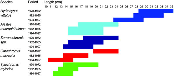
FIGURE 13. Length selectivity of dominant mesh sizes in the fishery with stationary gillnets of Lake Mweru for the five commercially most important target species. Mesh size changes from 102 mm in the 1970s via 76 mm in the 1980s to 63 mm in the 1990s. The top three species are all piscivores. Active methods with gillnets (seines, water beating) will change the size structure to larger specimens.

2. Fishing: the decrease in mesh size of the dominant gillnets in the fishery, as a result of decreased catch rates (Figure 12), changed fishing pressure to smaller length ranges and different species (Figures 11 and 12). From Figure 11 it can be inferred that the length of species in the commercial catch goes down, as a function of the dominantmesh size in the fishery. Length-selective pressure thus has changed to smaller sizes. Larger individuals of species can escape this fishery. This could be an explanation why larger Oreochromis mweruensis, mostly caught in nets of 102 mm and higher, increases in biomass despite increased effort: large Oreochromis escapes the present stationary gillnet fishery with 63 mm nets.^[11] However, this does not explain yet why the biomass of Oreochromis has increased in the first place, so that a larger stock of older year-classes could survive?

3. Change in productivity: peaks in recruitment need to occur occasionally to be able to trigger a situation where length-selective mortality incurred by the fishery (F = a proportion of the fishable biomass) will not lead to the subsequent early disappearance of a particular year class. Erratic recruitment with occasional extreme peaks will be an adaptive life history characteristics of a species, that will over time lead to a shift in the size structure not only of the individual species but also of the fish community. Large slow growing species with generally low recruitment levels will eventually disappear from a fishery even if they are fished with passive length-selective fishing methods. In other words: large specimens of such species do not necessarily have to be fished out themselves, their biomass will decrease through natural causes, not being supplemented by younger year-classes. In contrast, small fast-growing short-lived species, with highly fluctuating recruitment levels triggered by external drivers will always show extreme variability in catches and catch rates, independent of the size of the fishing mortality: they appear and die faster than the fishery can fish them out. But, and this is the point to be made, also larger species that have slower growth rates, and irregular recruitment -that is occasional extreme peaks - will show a high variability. In the case of pulsed systems like Mweru and Oreochromis mweruensis changing water levels triggers these peaks. This will result in considerable change in size structure within a few years after such events, despite high selective fishing pressure, as the fishery does not adapt as fast as the size-structure changes. For instance, two years after the high water levels in 1998, catches of 25 cm (? two year old), Oreochromis were so high that the two fish freezing factories stopped buying fish in fishing camps as their freezing capacity was too low to handle the enormous supply. A large increase in biomass of Oreochromis of 25 cm had occurred due to the recruitment peak in 1998 (van Zwieten, pers. obs.).

FIGURE 14. Catch rate composition of experimental gillnets in groups of four mesh sizes in three periods from 1970 to 1996. Shown are the six most important species in the catch and a rest group containing all other species. Solid and broken arrows indicate the first and the second dominant mesh size in the catch respectively. Blue in stacked bars represents fish predators.

6.3 Changes on a system level

Based on the three mechanisms that explain the overall changes in biomass-size structure of the Mweru fish community, we will now look at changes on a system level. A biomass-size curve of a fish community is exponentially descending over size: there is a larger biomass of small fish than large fish. Variations in the shape of this curve indicate systematic changes in the size-structure of a community that can be related to variables such as changes in lake-productivity and human impacts (Cyr, Downing and Peters, 1997). The first question is whether there is a systematic change in the overall distribution of length classes over biomass. Regression lines through a log-transformed biomass-size curve^[12] differ in slope and intercept with the biomass-axis, which differences can be interpreted as follows:

1. same slope but decreasing intercept means a decrease in overall productivity: this seems to have happened between the periods 1970/72 and 1982/85. Note that this means lower biomasses of smaller as well as larger sized fish.

2. increasing slope and increasing intercept means a shift of the biomass of a fish community towards smaller species and specimens (Rice and Gislason, 1996). This seems to have happened between 1972/85 and 1993/96.

Two questions are relevant for a decision on the significance of these observed differences. First, disregarding the distribution of the residuals around the regression lines, are the observed slopes and intercepts at all significantly different from each other? Second, it will be immediately clear from the graph (Figure 15) that the residuals are not randomly distributed around the regression lines, but are considerably auto-correlated, which has an influence on the values of both slope and intercept. What information does this curved shape of the distribution of the biomass-size structure of the community contain? Changes in the shape of the distribution are of interest, in the light of the above outlined model on changes in size structure on a species level (Figure 12). The first question will be answered by stepwise examining a series of regression models through which slopes and intercepts can be compared. The second question will be answered more tentatively by comparing the shapes of splines drawn through the three biomass-size distributions constrained such to explain at least 90 percent of the variation in the length-biomass distribution, and relate these splines both to changes in fishing and lake level fluctuations.

First: are the changes in slope and intercept as noted significant, in other words, are the perceived differences in intercept of 1990s > 1970s > 1980s and in the slope of 1990s > 1970s = 1980s? Slope and intercept of a regression line are strongly correlated, which means that they cannot be independently examined for significance between different regression lines. By examining the reduction in variability in regression models in which either slope or intercept are fixed, and compare these with the overall reduction of variability in the full model the significance of changes in intercept and slope can be established (Table 6). The amount of variability explained by the differences between slopes (r² = 0.02) and intercepts (r² = 0.03) in the full model is very small. The full model (the last line in Table 6) gives the result that the intercepts are significantly different only between 1990s and 1970s, while all slopes are significantly different from each other, with 1990s having both the highest slope and intercept. In the full model, the slopes of the 1970s and 1980s closely resemble each other, but separate slope analysis reveals that there is no difference between the three slopes. Co-variance analysis shows that only the intercepts of 1990s and 1970s are significantly different from each other, with higher intercept in the 1990s. The intercepts of the 1980s and 1970s are not significantly different from each other. From this analysis we can conclude that while a change in productivity between the 1970s and 1980s cannot be shown, the change in size distribution between the 1990s and 1970s is significant. This indicates that in the last two decades a qualitative change in length distribution of the whole fish community has taken place. But it is also clear from this analysis that the observed differences in overall size structure are not dramatic, when taking into account the large time window (>20 years) and the massive increase in fishing effort that has taken place over this period.

TABLE 6. Regression models to compare the significance of sources of variation explaining the total variation in the biomass over size. Both biomass and size were centred around the mean (mean L = 49.5, mean B=1.27). L = length (size); B = ¹⁰log(CpUE) (= biomass); D = decade, respectively top = 1970-72; middle = 1982-85; bottom = 1994-97; N_obs = number of obsevations corrected for the mean. SSQ = sum of squares; Df = degrees of freedom of the explanatory variable (source); significance levels are indicated by asterisks: * = p<0.05, ** = p<0.01, *** = p<0.001, n.s. = not significant

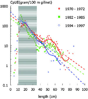
Second: what information can be inferred from changes in the shape of the biomass-size distribution? A clear dip in the length structure around 44 cm can be observed in the 1970s, decreasing to 36 cm in the 1980s. The dip disappears again in the 1990s. By then the descending curve is smoothed both through an increase in smaller size categories compared to 10 and 20 years before, and the disappearance of the peak in biomass around 51 cm (1970s) and 54 cm (1980s). In other words, it seems that between the first two decades a broadening of size selective mortality has occurred towards smaller fish, causing the plateau between 36 and 54 cm. Both 1970s and 1980s distributions were preceded by high water levels in 1968 and 1979 respectively or between 2-5 and 3-6 years before the periods over which the size distributions are calculated. Since 1986 up to 1998 water levels consistently decreased (Figure 9). The dominant fishing pressure was directed to fish species of up to 35 cm, shifting to smaller sizes over time (grey bar in Figure 15; Figure 13). Larger sized fish will be caught by active methods and by non-size selective processes such as entangling, which could have quite an effect taken over a whole fishery. However, these observations could also indicate that larger sized fish disappeared in the 1990s because of reduced pulses of productivity over a significant period of time. Increased biomass of smaller sizes in the 1990s could then occur both because of decreased predation pressure and fishing.

FIGURE 15 Biomass-size distribution with linear regression lines and spline by period. Splines were constrained at lambda = 100 explaining 91-92 percent of the variation. Linear regression was done from lengths ³ 14cm. The parameters from the linear regressions for respectively the 1970s, 1980s and 1990s are as follows (¹⁰log-transformed values): intercept = 2.52, 2.37 and 2.71; slope = -0.027, -0.029, -0.037; r² = 0.83, 0.68, 0.78. All slopes and intercepts were significant at p< 0.001, but see text for further explanation. Grey bar indicates selectivity of the gillnet fishery over the whole period between 1971 and 1997 of species of commercial importance.

As the conceptual model in Figure 12 indicates, a dip in the biomass-size structure followed by a peak at larger sizes could come about both through previous periods of higher productivity and because of size-selective fishing pressure. Size selective mortality through fishing did shift to the smaller species that have a higher turnover and hence are more resilient to this pressure. But it cannot be decided from just these observations alone which of the three processes are dominant in determining the particular shapes of the biomass size curve in each period. However, it will be clear from these tentative remarks that, while fishing will have an effect on size structure and species composition of fish community, fishing alone does not determine it in this system where large recruitment peaks occur as a result of irregular large (to extreme large) flood pulses.