4. RESULTS

4.1 Analysis of catch-rates

The time series analysed included one low water recession period with no fishery from 1996-1997. This recession occurred 33 years after the previous major recession in 1968, which was extensively documented in Kalk, McLachlan and Howard-Williams (1979). Another minor recession occurred in 1973-74. No catch-rate data are available for the years 1976 and 1977. The results of the analysis of variance and subsequent trend analysis are summarized in Table 2 and Figures 2 to 6.

4.2 Variability in catch-rates is extreme and possibly administratively induced

The variability in catch-rates, expressed as coefficient-of-variation (CV = standard deviation/mean) of the original (non-transformed) data, was extremely high. For instance catch-rates in gillnets, the series with lowest variance (variance = ¹⁰log(s²) = 0.14), the coefficient of variation can be estimated through CV= Ö(10^{2.303*variance} - 1) at 1.04. For other fisheries, daily catch variability (i.e. basic uncertainty as variability with trend and seasonality removed) expressed by CV ranges from 0.1 to 0.5 for trawlers to >1 in sport fisheries and some marine light fisheries. Therefore the aggregated monthly CV in the Chilwa data was about as high as the daily variability that individual sport fishermen experience (Densen, 2001). Individual gillnet fishermen experience a much lower day to day variability in catch-rates, with CV’s of around 0.5 to 0.8 (Densen, 2001). The extreme variability in the Chilwa data was even more surprising taking into consideration that the catch-rate series represented aggregations over strata, fishermen and month: the effect of aggregation is that variability is reduced. A dis-aggregation over month and fishermen to daily catch-rates would result in a coefficient-of-variation that is outside the experience even of fisheries exhibiting high daily variability, for example whale fishing (Densen, 2001), sport fishing on pikeperch (CV = 1.2, van Densen, 2001), and the Bagan light fishery on small marine pelagics in Ambon, Indonesia (CV = 2.4, Oostenbrugge, 2001). The variability in the Chilwa data is definitely outside the range of any gillnet or seine net fishery known from inland fisheries.

Apart from possible effects of trend and seasonality, discussed later, the extreme variability probably is caused by the method of raising the daily catch and effort data to arrive at the estimates of monthly catch and catch-rate. Conversion factors are used to arrive at estimated total catches per standard gear by stratum. After that the effort and estimated catch figures collected during the month are each added to obtain a total catch and total effort. The monthly catch-rate (CPUE) used in our analysis is calculated from these data. This summation procedure induces variability that is not present in the original data collected at the beach. Apart from that, the procedure makes it impossible to detect outliers and typing errors. In other words, much of the variability encountered in the Chilwa time series - and by extension the time series from other fisheries as the same system is used throughout Malawi - is “administratively induced error”. However, as the procedure has been maintained over the years, and there is no reason to believe that the administratively induced error changes over time (i.e. it can be considered random), it is still possible to proceed with our intended analyses of trends and their alleged causes. The enormous variability in the data has important consequences for the detection of trends and the analysis of causation: trends and fluctuations will be lost in “noise”, most of which unfortunately is administratively induced.

4.3 All gears except traps are selective

The variation in total catch-rates was lowest in gillnets with a factor^[19] (F) around the geometric mean of F = 5.6 followed by traps (F = 9.4), seines (F = 16.9) and longlines (F = 20.3) (Table 2, Figure 2). On a species level lowest variation is seen in Oreochromis shiranus (F = 7.6) and Clarias gariepinus (F = 6.5) in gillnet catch-rates. For most other species-and gear combinations the variation is around a factor 20 or higher. Aggregation of catch over species thus leads to a reduction in variation. However, only in traps does the aggregation of various species to total catches lead to a significant reduction in variation. This indicates that it is the only truly “multispecies” gear in its target: all species are caught in more or less the same amounts over the same period of time. The main target for gillnets is O. shiranus, for a seine is Barbus paludinosus and to a lesser extent O. shiranus, while longlines target C. gariepinus. Other non-target species only reduce the variance in total catches slightly. In the case of longlines this reduction of F is just three percent.

4.4 Annual variability is high

Annual variability in catch-rates was high, and significant inter-annual differences explained much of the total variance (Table 2, Figures 2 and 3). As a result the unexplained factor around the mean was lowered by 50 - 75 percent in 14 out of 20 cases. In the remaining six cases, which were all non-target species for the various gears, no variation at all could be explained by temporal analysis, and catch-rate data of these species-gear combinations on the aggregated level of the lake by month indicated pure chance.

FIGURE 2. The amount of variability expressed as factor around the geometric mean explained by trends (as linear regression), annual, monthly and residual variation. The residual variation is also expressed as standard deviation (s) at the bottom of each column. The arrow indicates the target species of a gear. Basic uncertainty (see text) is the variability remaining when trend and seasonality are subtracted from the total variation.

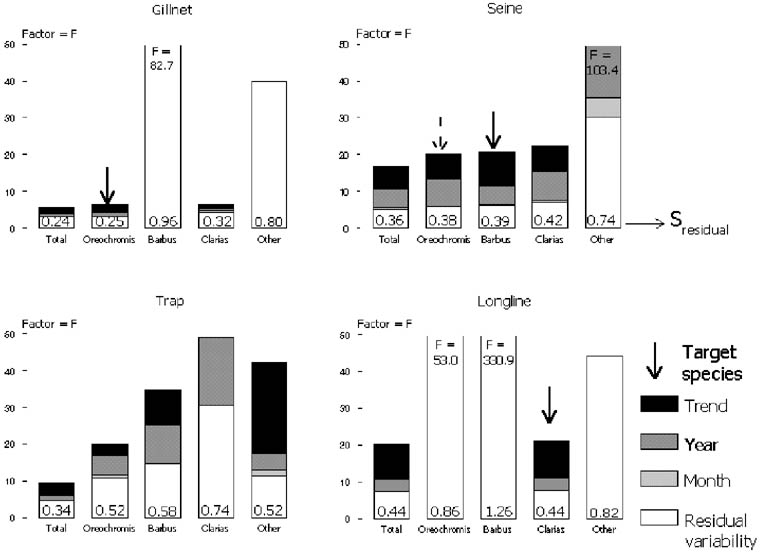
TABLE 2. Results of Analysis of Variance and regression analysis on monthly catch-rates of Lake Chilwa by gear and species groups as contained in the CEDRS of Malawi (see text for further explanation)

Significance level is indicated by asterixes: * p< = 0.05, ** p< = 0.01, ***p< = 0.001

FIGURE 3. Annual variation in total catch-rates by gear. Vertical bars represent 95 percent confidence limits. Note ¹⁰log scale on vertical axes.

FIGURE 4. Monthly variation in total catch-rates by gear. Vertical bars represent 95 percent confidence limits. The scale on vertical axes represents a multiplication factor of the of the ¹⁰log annual mean catch-rates.

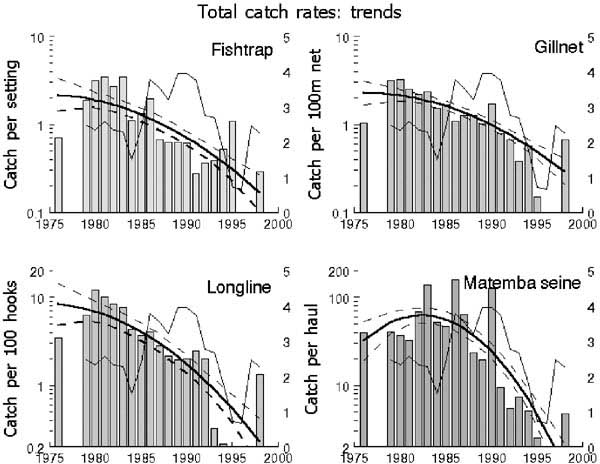
FIGURE 5. Annual variation (bars) and polynomial trends (thick line) in geometric mean annual total catch-rates by gear in lake Chilwa. Trends are shown with 95 percent confidence limits (broken lines). The thin line is the relative mean annual water level of the lake.

4.5 No seasonality is present

Generally, no seasonality was observed in the catch-rate data, as no significant differences between months were found in 14 out of 20 series. This indicates that the catch-rate data do not contain a clear seasonal signal for most species(groups) examined (Table 2, Figure 4). Significant differences between months were found in six cases: of Oreochromis and of “Other” species caught in fish traps; of Clarias caught in Matemba seines and in gillnets; of “Other” species caught in Matemba seines; and in Matemba seines on the aggregated level of total catches. The clearest seasonal signal was seen in traps where 11% of the total variation in catch-rates is explained by the significant differences between months. Overall catch-rates of Oreochromis are higher from January to April during rising water levels (Figure 10), however only May, July and December had significantly lower catch-rates compared to the months February to April. “Other” species had significantly lower catch-rates in December and January, the season with lowest water levels, compared to the remaining year. But only 7% of the total variation was explained by this difference. Clarias catch-rates of Gillnets and Matemba seines were slightly elevated during the low water period in December and January, which explained 10% and 6% of the total variation. Differences between monthly catches of “Other” species in Matemba seines explained only six percent of the total variation, and were caused by lowered catch in December compared to the period between March to June and October. On an aggregated level by gear only Matemba seines showed monthly differences: February was slightly elevated compared to much of the period from June to December, but the signal was weak as it explained merely 5 percent of the total variation.

4.6 All observed trends are declining

All but six out of 20 time-series revealed a substantial downward trend in average catch-rates ranging in speed from a factor 4 in Clarias catch-rates of gillnets to a dramatic factor 120 in catch-rates of “Other” species in fish traps (Table 2, Figures 5 and 6). Polynomial trends indicated that all of the downward trend legs of the curves commenced before 1986 and most even before 1982. Trends were linear or concave downward in ten series. The quadratic term of only two of the seven concave downward series contributed more than 10 percent to the total variation explained by the trend, indicating that the linear downward component was dominant in all cases. Four series had a dome shaped trend, but with just a slight upward slope and a strong downward slope after the peak. Three of the peaks within these four series were in 1982 (total catches in Matemba seine), 1983 and 1984 (Oreochromis catches in fish traps and Matemba seine). “Other” species caught in Matemba seines peaked in 1986 and this was the only series without a linear component. Thus most of the downward trends could be sufficiently explained by the linear component and the remaining analysis will be done using linear trends.

FIGURE 6. Annual variation (bars) and polynomial trends (thick line) in geometric mean annual catch-rates by species and by gear in lake Chilwa. Trends are shown with 95 percent confidence limits (broke lines). The thin line is the relative mean annual water level of the lake.

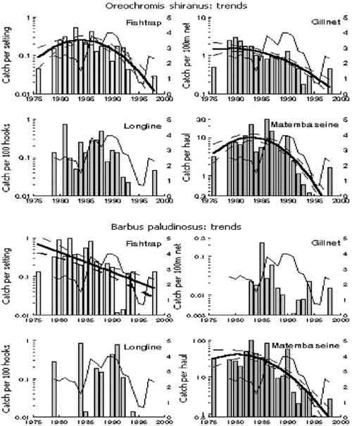
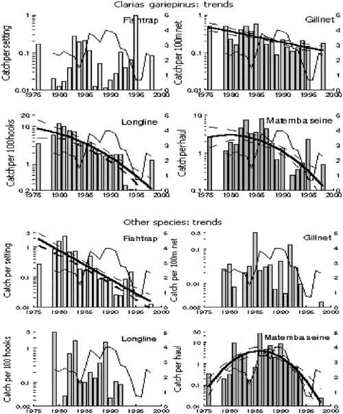
The trend component in the variation is strong: 44 percent to 88 percent of the observed annual variation was explained by the downward trends (Table 2, Figure 2). Both for fish traps -except in case of Barbus - gillnets and longlines more than 60 percent of the annual variation was explained by trends. The highest amount of total variation explained by a linear trend was in “Other” species caught by fish traps (40 percent). Linear trends in total catch-rates explained between 27 percent (seines) and 36 percent (gillnets) of the variation.

4.7 Basic uncertainty is high

Unexplained variation is the amount of variation that remains after all significant year and month effects (trends) are subtracted from the monthly catch-rate time-series. The unexplained variation is lowest in gillnets (F = 3.1), followed by fish traps (F = 4.8), seines (F = 5.2) and Longlines (F = 7.6). Except in traps, the unexplained variation is about the same or somewhat higher for the separate target species of the various gears compared to the total catch-rates (Table 2, Figure 2). The basic uncertainty, or the uncertainty remaining after removing the trend, is a factor F = 4 for gillnets and F = 6.5 for traps. Basic uncertainty in catch-rates of seines and longlines is excessively high (F = 11), indicating strong interannual variation.

TABLE 3. Trend, trend-to-noise ratio and number of months data needed to detect the observed trends with and without autocorrelation (persistence).

4.8 Trend-to-noise: the capacity to detect trends

All linear downward trends were detectable as statistically significant between 19 and 24 months for the total catch-rates of the four gears (Table 3, Figure 7). Persistence (= non-random residuals) had little effect: it increased the number of data points needed to detect the observed trends with two to three months (Figure 7). Trend-to-noise ratio was highest in “Other” species in traps, and lowest in Barbus caught by traps. The effect of persistence in the species(groups) was an increase in the data points needed, but all observed trends were detectable from 21 to 38 months of data.

A long-term negative trend for total catch-rates in gillnets and longlines became statistically significant in 1987 (Figure 8a), in both cases around seven years after the peak in catch-rates was reached (Figure 5). The negative trend in fish traps was significant in 1988, or around five years after the peak. Matemba seines gave a different signal: the negative trend was significant in 1992 or around two, six and nine years after peaks observed in average annual catch-rates and about nine years after the estimated peak in catch-rates through polynomial regression (Figure 5). Reversals in trends seen in all catch-rate time-series took about three to four years during which only the decision of no long-term trend could be made. For example, this was the case from 1984 to 1986 in gillnets (Figure 8a).

Short-term trends, taken over five years, are obviously much more erratic (Figure 8b), but nevertheless gave fairly consistent signals over time. For instance a strong positive trend (b/s = 0.88) seen in 1980 after three years (plus two missing years) of gillnet data, reversed into a fairly strong negative trend (b/s = -0.40) in 1981. From 1981 to 1988 the short-term trends remained negative, though becoming less strong. Between 1988 and 1991 no short-term trends were seen. During this period of higher water levels, catch-rates levelled out (Figure 5 and Figure 9A). After that short-term trends became significant and negative again. This picture is confused by the behaviour of short-term trends in other gears. Fish traps and longlines did not exhibit negative short-term trends until after 1983 and Matemba seines not even before 1989. Short-term trends in fish traps remained negative until 1995 the year before the lake dried up, while all other short-term trends remained negative until the end of the series in 1998. Furthermore, reversals in short-term trends take place more often in these gears and result in relatively high absolute values of the trend-to-noise ratio.

FIGURE 7. The relation of the trend-to-noise ratio to the number of months of data needed to detect a trend in total catch-rates and catch-rates by species/gear combinations of including the effect of autocorrelation (persistence)

FIGURE 8 A. Development of the trend-to-noise ratio from five years of catch-rate data in 1980 onwards with successive addition by year of monthly catch-rate data for gillnets, Matemba seines, fish traps and longlines. 1980 is the trend-to-noise over 1976 to 1980; 1981 is b/s of 1977 - 1981 etc. B. Development of trend-to-noise over five year moving periods, each indicated by the last year

4.9 Water levels, fishing effort and catch-rates: immediate effect of changes in water level on catch-rates

Average annual water levels increased significantly from 1986 to 1991 compared to the periods before and after. Water levels dropped from 1992 onwards to the drought of 1995 and 1996 when the lake was largely dry. After that the average water level increased to pre-1986 levels (Figure 9). This means that during the period over which we have data on catch-rates (1979-1998) a significant fluctuation in water levels took place providing the necessary contrast to detect the effect of increased effort with changing water levels. In all cases except catch-rates of “Other” species in Matemba seines, which peaked in 1986, catch-rates peaked before the onset of the higher water levels. This can be clearly seen in Figures 5 and 6.

Changing water levels have, in all but one case, an “immediate” effect on annual average catch-rates: fluctuations in water levels are reflected in the same or the following year in the catch-rate levels (Table 4). De-trended annual catch-rates in gillnets positively correlated best with either mean or maximum average lake levels and significant lags varied between zero years for O. shiranus in gillnets and seine nets, to four years for C.gariepinus in seine nets. In contrast, regressions between catch-rates by species or gear and water levels with lags higher than one year were not significant, except for total catch-rates in seines. The correlations indicating long-term effects of water levels on catch-rates (i.e. inducing generations of strong and weak year classes of longer lived species) are thus rather weak signals in the variation in catch-rates as observed through the CEDRS data.

FIGURE 9. A. Annual average water level (thick line) and mean monthly water levels (thin line) in Lake Chilwa from 1979 onwards. B. Long term average monthly water levels and minimum (excluding periods of recession) and maximum water levels measured by month

TABLE 4. Cross-correlation between residuals of de-trended annual average catch-rates (“anomalies”) and annual mean, minimum and maximum water levels in Lake Chilwa. Analysis is done on total catch-rates by gear and the main target species (groups) of the various gears. Trend is a linear regression on annual average catch-rates. Regressions of anomalies on water levels are done on lags with the highest significant correlation. N = number of observations, r² = proportion of explained variation, b = trend parameter. Significance values are denoted by asterixes: * p<0.05, ** p<0.01, *** p<0.001

Where an effect of water level on catch-rate could be detected, it explained 10 percent to 40 percent of the total variation in annual average catch-rates. Approximately 23 percent of the residual catch-rates of gillnets (amounting to approximately 14 percent of the total annual variation) and 36 percent of the residual catch-rates of O. shiranus in seines (= 22 percent of total variation) were explained by the mean water level of previous years. In all other cases, the highest significant regressions between the residual catch-rates were found with “this year’s” maximum water levels, which in case of O. shiranus in Matemba seines amounted to 63 percent of the residual variation (= 40 percent of total variation) explained. Residuals in total catch-rates in Matemba seines were explained for 22 percent by the average water level of one year earlier (»10 percent of the total variation).

4.10 Effort increases fast and is population driven

All indicators of fishing effort increased significantly over the period examined: i.e. number of gear owners, assistants, boats and gears. Trends in numbers of gear owners, assistants, boats, gillnets and longlines indicate a three-fold increase while, traps and Matemba seines increased five fold (Figure 10). In the 1980s the number of fishing operators - gear owners and ancillary workers - in Lake Chilwa ranged from 2 060 to 3 403 while the range was from 3 955 to 9 466 in 1998, just two years after refilling of the lake (Table 5). This latter figure represents the highest number of fishermen and assistants ever registered on Lake Chilwa. Apparently many new fishermen entered the fishery after the recession, mainly in the west and north. This increase could be attributed to return migration from South Africa due to phasing out of the working contracts in the mines. We assume that many of the returning migrants took up fishing, as the Phalombe plain does not receive much rain making agriculture around the upland area an unattractive option.

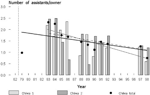
All gears, both the low-investment (traps, longlines and handlines) as well as high-investment gears such as Matemba seines, continuously increase in units over the years. However, as the ratio of gear owners to assistants as well as number of boats and gears per owner exhibit a steady decrease over the period from 1983 to 1998 it is likely that low investment gears (traps, longlines, and nchomanga) become relatively more popular (Figure 11).

FIGURE 10. Development in effort expressed as number of gear owners, number of assistants and number of boats in Lake Chilwa. The bold line is the regression of the total numbers over time. The thin regression line refers to the numbers of stratum 1 and the broken line is the regression of numbers of stratum 2 over time.

Most fishing effort is suspended during recession periods. Many fishermen, especially those operating Matemba seines and gillnets, stop fishing or migrate to other water bodies, though such migrations recently have encountered resistance from resident fishermen (Njaya, pers. obs.). Other fishermen migrate to pools of water remaining in the inflowing rivers. Fishermen operating fish traps sometimes set their traps in rivers, often in conjunction with weirs.

4.11 Increased effort negatively affects catch-rates despite high regenerative capacity

We concluded in the previous section that a significant part of the variation in catch-rates is immediately explained by absolute water levels. This implies that catch-rates should increase with higher water levels and vice versa. However, between 1984 and 1991, with elevated water levels, no positive short term-trends were observed though trends became less strongly negative over time or indicated stable levels (Figure 8b). Long-term trends reveal a stabilization in catch-rates between 1984 and 1987 for gillnets, fish traps and longlines and between 1988 and 1991 for Matemba seines (Figure 8a). This would imply that the expected downward trend observed in catch-rates is delayed by increase in production during high water levels. After 1992, during the years before the recession, increased effort and decreasing water levels push stocks in the same direction, as a result of which the decrease in catch-rates will probably accelerate compared to a situation with low effort levels. However, closer examination of the trends versus catch-rates (Figures 5 and 6) show an increase for species (groups) caught in fish traps and for Clarias gariepinus caught in Matemba seines in the two to three years before the complete recession, thus confounding the explanations on the general trend.

Multiple regression of water levels and catch-rates confirms these observations: in all cases fishing effort had a significant negative effect on catch-rates. In gillnets 26-40 percent of the variation in annual catch-rates was explained by the number of gillnets for both Oreochromis and Clarias; in seines this amounted to 52-56 percent for all three species; longline effort explained 57 percent of the variation in annual catch-rates in Clarias. In traps the highest significant effect was found with Clarias (47 percent), while effort explained only 16 percent in Oreochromis catch-rates (Table 6). Water level was positively related to annual catch-rates, but explained much less than fishing effort (7-29 percent). In all gears, except longlines, Oreochromis catch-rates were affected most by water levels (20-29 percent). Clarias catch-rates were only significantly influenced in seines (15 percent) and longlines (7 percent), but not in gillnets and traps. Barbus catch-rates were only influenced by water level in seines (13 percent), but otherwise the regression model could not explain variation in catch-rates of Barbus.

TABLE 5. Number of fishermen, ancillary workers and craft operating in Lake Chilwa (1984-98)

Source: Fisheries Department Frame Survey (1984-98)

FIGURE 11. Ratio of number of assistants and gear owners. The bold line is the regression of the total numbers over time. The thin regression line refers to the numbers of stratum 1 and the broken line is the regression of numbers of stratum 2 over time.

4.12 Efficiency of gears (catchability) increases with decreasing water levels

The interaction of water level and gears was significant and positively related to catch-rates, except with seines. The lowest number of gears, counted at the beginning of the time series, as well as the highest number of gears at the end of the series coincided with low water levels, while highest water levels around 1990 are associated with a period of increasing fishing effort with all gears. The drop in water level towards the recession in 1996 and 1997 is thus associated with the highest numbers of gears counted in the time series of fishing effort. Theoretically increased fishing effort would be associated with decreased catch-rates. However, the high proportion of variation explained by the interaction term indicates that the situation is more complex. During receding waters, with a likely subsequent concentration of the fish, some of the gears catch a number of species more efficiently thus maintaining relatively high catch-rates despite increasing effort. This is the case with Oreochromis caught with gillnets (30 percent of variation explained by interaction term) and traps (21 percent), and with Clarias caught in gillnets (29 percent), traps (26 percent), longlines (18 percent) and to a lesser extent seines (7 percent). This sustains the notion of a crowding effect of these two species during receding water levels. It is particularly clear in the case of Clarias where relatively high catch-rates are encountered during very low water levels (Figure 6). There are indications that Clarias become more “active” under extreme low water levels in an attempt to find their way out of the desiccating areas changing their catchability.

That the interaction effect does not play the same role in the case of Matemba seines may not be surprising. Seines are active gears used either from the shore, or from boats in and around submerged vegetation, in relatively shallow areas. They are used both with receding or increasing lake levels in the areas where concentrations of smaller species and juveniles of larger species are found. Changes in recruitment levels will therefore affect catch-rates more than crowding effects, which is indicated by the high explanatory value of the water level in the statistical model where seining effort is the explanatory variable. In comparison, longlines show the reverse situation: in this case recruitment variation is much less important (7 percent of variation explained by the effect of water level) compared to the interaction effect (18 percent). Of all gears, the increase in effort of seines and longline explains the highest proportion of variation in their respective catch-rates, indicating a comparatively strong effect on stocks.

TABLE 6. Proportion of variation in annual catch-rates explained by the multiple regression model with lake water level (mean, minimum or maximum), with or without a lag phase of 1 year, fishing effort (number of gear) and their interaction as explanatory variables. Sign indicates the direction of the effect in the model. Left of the vertical line are the statistics of the multiple regression model. Analysis is done on total catch-rates by gear and the main target species (groups) of the various gears. Only regression models explaining the highest amount of variation are shown. Df = degrees of freedom, SS = sum of squares, % = r² = proportion of explained variation, sign denotes the direction of the effect in the statistical model. Significance values are denoted by asterixes: * p<0.05, ** p<0.01, *** p<0.001