![]()
![]()
![]()
The ability to simulate and predict over time the fate of organic materials added to the soil,whether by litter or by additions of crop residues and organic manures through crop and land management,is fundamental to carbon accounting and to the formulation of scenarios of land use and LUC that may increase carbon sequestration.
Methods for estimating and measuring changes and fluxes in SOC can be direct or indirect.
Direct methods include:
field sampling and laboratory measurement,
C (CO2) flux monitoring.
Indirect methods are:
accounting (including stratified accounting),
modelling (simulation).
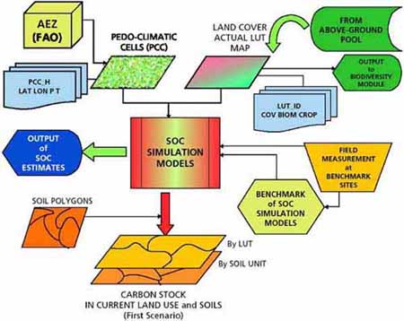
FIGURE 7 - Estimation of carbon stock in current land use and soils (belowground pool) through simulation modelling
In the developing world, the costs, instrumentation requirements, labour intensity and technical knowledge involved in implementing direct methods for routine practice set them out of reach (aside from specific research projects). Therefore, they are not the concern of this report. Accounting methods are described at length throughout this document. Accounting also takes into consideration the strata generated by land cover classes derived from satellite imagery and air-photo interpretation. Modelling can be thought of as an indirect method for estimating changes in SOC. However, it is within reach of standard practice in the developing world, provided the data sets to feed into the model are available from resource inventories.
Carbon stock in soils under present land use can be estimated through carbon dynamics simulation models. The prerequisites for model implementation are:
the objects of modelling, i.e. the pedo-climatic cell (PCC) or soil polygon whose carbon dynamics are to be simulated. These units may be the result of zoning or partition of the environment into units.
knowledge of the model, its structure and operation.
the model data requirements. These determine the input data set and the difficulties in model parameterization.
Figure 7 illustrates the use of simulation models in the estimation of carbon stock under current land use.
The dynamics of C in the soil are complex. Accordingly, the models that simulate these dynamic processes can be complex too. Soil carbon simulation models are process-oriented multicompartment models. Typically, the models are mainly empirical in nature and all contain a slow or inert pool of organic C, which is not necessarily described in its nature or rate of formation. Some models treat the soil as homogeneous with respect to depth. Usually, the nature of litter is treated as being different to that of SOM. Many of these models reveal convergence in kinetic compartmentalization and a growing use of clay content and the inclusion of an IOM component.
As Figure 7 shows, the selection of the object of modelling (PCC, ecological zone or soil polygon) results from a process of partitioning the spatial variability of environmental parameters, soils, climate, landscape, etc. These procedures are discussed in later sections. Land cover classification and mapping, and the selection of quadrat sampling sites to serve as benchmarks to the model calibration, are discussed above. Thus, the following section focuses on model selection.
Simulation models vary in their degree of complexity and other attributes relevant for model selection by technical staff. Reports on the use of carbon simulation models are relatively abundant in the specialized literature (e.g. Smith et al., 1997b; Coleman and Jenkinson, 1995b; Powlson, Smith and Smith, 1996; Li et al., 1997; Izurralde et al., 1996). The characteristics of such models vary in terms of their emphasis on some particular aspects of the carbon cycle, their degree of compartmentalization, the underlying assumptions made by the developers of the model, model performance, their required inputs, nature of outputs, accessibility and ease of use.
A number of comparative studies and evaluation of simulation models have been reported. Smith et al. (1997b) compared the performance of nine SOM models using data sets from long-term experiments. The models, referred to by their acronyms, were: RothC, CENTURY, CANDY, DNDC, DAISY, NCSOIL, SOMM, ITE and Verberne. Smith and coworkers observed that not all models could simulate all data sets, and that only four models attempted all. No one model performed better than all others across all data sets. The first six models (i.e. RothC, CENTURY, CANDY, DNDC, DAISY and NCSOIL) performed with no significant differences in accuracy between them. They predicted with significantly less error than the other models in the list.
Izurralde et al. (1996) evaluated five models (CENTURY, RothC, SOCRATES, EPIC and DNDC) in terms of their performance and a number of other parameters, at site-specific scale and at ecodistrict level in Alberta, Canada. SOCRATES appeared to be their choice because of its ease of operation and ability to mimic long-term trends. However, they concluded that for modelling regional carbon storage this model may be limited by the lack of detailed management options. CENTURY predicted long-term trends reasonably well and had more management options - management being a deciding factor in the nature of carbon fluxes in soils.
The European Soil Organic Matter Network (SOMNET) published a systematic review of simulation models (Smith et al., 1997a). This can be consulted on line via the Internet (http://saffron.rothamsted.bbsrc.ac.uk/cgi-bin/somnet-models).
Selection of a carbon simulation model
The Internet resources of SOMNET offer a comprehensive list of models and a detailed description of the characteristics of each model, their required inputs, outputs and the conditions within which the model has performed best. It is beyond the scope of this report to offer a summary of such listings. In order to make a selection of the final model to be used for estimating changes in SOM and SOC over time, the reader is advised to: (i) access the Web site; (ii) decide on the criteria for selection of the model; (iii) narrow down, iteratively, to a short list of three or four models; and (iv) search for more detailed information about the model in the technical literature. Selection criteria could include:
the required inputs for the model ought to match available data in the databases.
the output variables generated by the model need to satisfy the objectives of the modelling exercise.
the model should have been adapted to the particular conditions of soil, climate and land management of the site or region.
the simulation model should offer the management options that need to be modelled.
the level of accuracy of estimates from the model should be within the target accuracy required by the project.
there is reported evidence that the model has performed well in ecological circumstances similar to those of the site of concern.
accessibility and ease of use together with the implicit assumptions in the model about the user’s technical background.
The models CENTURY and RothC-26.3 were selected in this project for simulating the dynamics of SOC and SOM turnover in the sites of the three case studies presented. The rationale for these choices was as follows. These models represent extremes of a gradient of accessibility, ease of use and complexity, CENTURY being the most complete. Although originally developed and tested in temperate conditions, both have been upgraded to encompass a wide range of ecosystemic variability, including tropical and subtropical conditions, which are present in a large part of Latin America and the Caribbean region. Moreover, both models are well documented and there is a sufficient volume of published work with the applications of both models to data. CENTURY is one of the most complete and frequently reported in studies of carbon dynamics simulation. Tables 6 and 7 show a summary description of the models as per SOMNET.
|
1. MODEL: CENTURY 2. MODEL NAME: CENTURY 3. SPATIAL SCALE OF THE MODEL Plot, field, regional, national, global 4. INTEGRATION TIME-STEP OF THE MODEL Months 5. DATA USED TO RUN THE MODEL a) Weather data used to run the model:
b) Soil data used to run the model:
c) Plant and animal inputs used to run the model: plant production data useful for testing the plant model d) Land use and management inputs used to run the model:
6. MODEL OUTPUTS a) Soil outputs:
b) Plant outputs:
c) Animal outputs:
d) Other outputs 7. MODEL DESCRIPTION a) Description of the decomposition of plant and animal debris: Decomposition of plant and animal debris described by multiple pools as follows:
b) Description of the decomposition of SOM: decomposition of SOM described by multiple pools as follows:
c) Factors assumed to affect organic matter decomposition:
d) Soil layers used in the model: the model divides the soil into one layer as follows:
8. MODEL EVALUATION Sensitivity analyses have been performed as follows: impact of changing initial soil C levels and temperature effect on decomposition has been evaluated. Model output has been compared to measured data that were independent of the data used in model development. Model output has been compared to measured data quantitatively arbitrary criteria have been used to define good model performance as follows: 95 percent confidence limits (Parton and Rasmussen, 1994). Good model performance has been defined by simulated results falling within the standard error or standard deviation of the measured data. Statistical methods are used to determine good model performance. as follows: SOM levels and plant production were compared to predicted values from regression equations (Parton et al., 1987). The model has met the criteria for good model performance in the following ecosystems / climate regions:
(Parton & Rasmussen, 1994; Paustian, Parton and Persson, 1992; Sanford et al., 1991; Parton, Woomer and Martin, 1994; Schimel et al., 1994) 9. USING THE MODEL
|
|
1. MODEL: RothC-26.3 2. MODEL NAME: RothC-26.3 Most recent version 26.3 3. SPATIAL SCALE OF THE MODEL Plot, field, catchment, regional, national, global. 4. INTEGRATION TIME-STEP OF THE MODEL Months 5. DATA USED TO RUN THE MODEL a) Weather data used to run the model:
b) Soil data used to run the model:
c) Plant and animal inputs used to run the model:
d) Land use and management inputs used to run the model:
6. MODEL OUTPUTS a) Soil outputs:
b) Plant outputs 7. MODEL DESCRIPTION a) Description of the decomposition of plant and animal debris: decomposition of plant and animal debris described by multiple pools as follows:
b) Description of the decomposition of SOM: Decomposition of SOM described by multiple pools as follows:
c) Factors assumed to affect organic matter decomposition:
d) Soil layers used in the model:
8. MODEL EVALUATION Model output has been compared to measured data which were independent of the data used in model development Model output has been compared to measured data quantitatively Good model performance has been defined by simulated results falling within the standard error or standard deviation of the measured data Statistical methods are used to determine good model performance. as follows: see references The model has met the criteria for good model performance in the following ecosystems / climate regions:
Possibly also cold and warm temperate and tropical forestry. Undisturbed natural vegetation in Broadbalk and Geescroft wilderness The model failed to meet the criteria for good model performance in the following ecosystems / climate regions: wetlands, all climate zones 9) USING THE MODEL
|
Model parameterization - preparation of soil and climate parameters
The models require three sets of data:
soil data,
climate data,
management data, including crop and land management and additions of organic materials in quantities and over time.
In order to derive the specific sets of variables to parameterize the models, the suggested methodology describes a set of procedures for the definition of agro-ecological zones (AEZs). These are essentially relatively homogeneous areas with unique combinations of soil and climate. They are referred to as PCCs. The characterization of the area is made in terms of AEZs following the FAO approach as describedbelow.
Biophysical characterization of the area
The biophysical characterization of the area is to be done in terms of thematic layers of information on soils, climate and land cover or land use. The cartographic representation of these data is at a scale adapted to the size of the study area or river basin. Typically, most countries within the Latin America and Caribbean region would have thematic coverages from past surveys and resource inventories. An appropriate scale for working at the level of a medium-sized watershed or basin would be between 1:20 000 and 1:50 000. At this range of scales, there is adequate detail on terrain conditions of the study area. The use of maps at this scale in countries such as in Mexico, for example, has an added advantage in that the official mapping agency, the National Institute of Statistics, Geography and Information (INEGI), provides coverage for 70 percent of the country at this scale. Application of these methods in other Latin American countries will require the use of similar map products that typically should include information on:
soil texture (clay and sand contents),
soil bulk density,
soil depth,
present land use.
In the process of biophysical characterization, two possible situations may occur:
the necessary information is present in digital format. Relevant information can be processed using a GIS. In this case, the GIS can help in generating the PCCs.
data are in analogue (non-digital) format, e.g. paper, plastic or other material. The PCCs need to be defined.
The latter situation will require a process of boundary definition through thematic overlay. Where this is achieved manually, some advantages can be taken of the situation in order to enhance data preparation of data for modelling. The following are some activities in the manual preparation of data:
1. definition of basin boundaries on a transparent or translucent surface - in such a way that when comparing it to the thematic maps the boundaries can be generated as required.
2. overlay of the map of present land-use classes on the map of vegetation cover (where these are two different maps) in order to eliminate sites without possibilities of carbon sequestration (i.e. urban, peri-urban and industrial areas). The map generated is to be considered the base map.
3. soil map. When overlaying the base map (Step 2) on soil boundaries, information such as the textural classes (i.e. the percentage of clay and sand), soil depth and soil bulk density can be extracted.
4. topographic map and its slope classes. The overlay of the topographic map on the base map allows the delineation of zones with slopes whose ranges determine the feasibility of certain activities. For example, the interval from 0 to 8 percent shows areas of the landscape where intensive agriculture can take place. From 8 to 30 percent slope, rainfed agriculture and the production of fruit trees is possible, and slopes greater than 30 percent would indicate areas suitable for forest systems. The resulting map provides a reclassification of slope ranges related to possible use.
5. the overlay of all of the maps produced in this fashion (i.e. Steps 2, 3, and 4) would generate a preliminary map of AEZs or ecozones or regions, as internally homogenous as possible in terms of relief, present land use and soil characteristics.
6. definition of AEZs or PCCs. Meteorological station values of climate parameters relevant to land use, such as length of growing period (LGP), moisture available in the soil, air temperature and radiation should then be upscaled in the same map base. Given that their position on the landscape is known through their coordinate pairs, it would be possible to identify areas of influence or “domains” of each meteorological station (e.g. Thiessen polygons). In these domains, it should be possible to obtain or extract values of climate parameters necessary for modelling. Where spatial data have been digitized and the spatial databases of resources are available in digital form, spatial interpolation techniques, such as kriging, bicubic splines or distance functions, can be applied. Interpolation or tesselation will be achieved automatically in GIS, such as indicated in Figure 8. The end of this stage achieves the definition of agro-ecological (i.e. pedo-climatic) cells that can be grouped into zones.
FIGURE 8 - Extraction of soil and climate parameters from agro-ecological cells or polygons for model parameterization
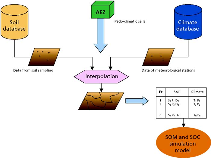
Preparation of soil and climate parameter data
This section explains procedures for preparing data to parameterize the simulation models (where databases of soil and climate are present).
In any given watershed, a database of soil characteristics may be present from past surveys and databases. Such databases may include records of soil samples and analytical data in any given zone, with the parameters required by the models (specified for each model). However, part of this information is often missing. In such circumstances, estimates of the values of the missing data have to be generated. A climate database may be generated with information from the meteorological stations that influence each zone, and whose location is nearest to the zone. The pooled values from such stations, although not strictly within the study area, may have to suffice for modelling purposes where insufficient stations fall within it.
Figure 8 illustrates how the PCCs or zones are to be characterized with data as accurate as possible, from soil profiles and from meteorological stations. For interpolation of these data, tables of attributes by each ecozone serve as the source of inputs to the SOM simulation models.
Model parameterization and calibration with site information
In order to parameterize the models, once PCCs or zones have been defined and identified, it is important to ensure that the data extracted from the databases of the PCCs provide the necessary variables to run the models. Therefore, before running the models an intensive data preparation stage should be planned and implemented carefully.
Data on the amount of organic matter, clay content (percent), bulk density and depth with regard to the soil profiles must be included. The contributions of the aboveground biomass to the soil according to the LUT and its management, in the form of crop residues, organic manures and litter, should be recorded and prepared for input into the models. The amounts of inputs of organic materials must be quantified in terms of tonnes of C per hectare per year.
Other important information needed for full model parameterization includes:
identification of areas where there are additions of crop residues, organic manures or any other organic material.
agricultural production by type of crop (Pai).
harvest coefficients (the percentage of the total biomass that is harvested) (Cci).
carbon-nitrogen ratio by species present in the crop mix.
moisture content in plant tissue by species (percentage of water in plant) (Hi).
production of forage per hectare (including roots) (F).
number of head of livestock in the grazing or pasture management unit, by species by hectare (Nci).
crop residues including roots, as percentage of total plant biomass (Eai). (The percentage of the plant that is removed as crop residues including roots if any. Where this information is not available, methods used in the calculation of the belowground biomass in this report can be used to derive an estimate.)
nutritional content of forage by species, or nutrition conversion index, which is a measure of the nutritional quality of forage (ICAi).
index or coefficient of grazing (R).
aboveground biomass and carbon content of annual herbaceous species (these data are obtained from the quadrat (1 × 1 m) sampling sites during the multipurpose field surveys) (Bh).
Simulation modelling of carbon dynamics in soils
This section outlines the specific procedures for running each of the SOC models selected. It discusses the requirements, characteristics and data for model input.
Modelling with RothC-26.3
Model characteristics
RothC-26.3 is a model of the turnover of organic C in non-waterlogged soils that allows for the effects of soil type, temperature, moisture content and plant cover on the turnover process. It uses a monthly time step to calculate total organic C (tonnes per hectare), microbial biomass C (tonnes per hectare) and D14C (from which the radiocarbon age of the soil can be calculated) on a time scale of years to centuries (Jenkinson et al., 1987; Jenkinson, 1990; Jenkinson, Adams and Wild, 1991; Jenkinson et al., 1992; Jenkinson and Coleman, 1994). It needs few inputs and these are easily obtainable. It is an extension of the earlier model described by Jenkinson and Rayner (1977) and by Hart(1984).
RothC-26.3 computes the changes in organic C as it is partitioned into five basic compartments: inert organic matter (IOM), decomposable plant material (DPM), resistant plant material (RPM), microbial biomass (BIO) and humified organic matter (HUM).
Input variables required to run the model
Table 7 indicates the data required to run the model. In particular:
rainfall and open pan evaporation are used to calculate topsoil moisture deficit (TSMD), as it is easier to obtain rainfall and pan evaporation data, from which the TSMD is calculated, than monthly measurements of the actual topsoil water deficit.
the air temperature (in degrees Celsius) is used rather than soil temperature because it is more easily obtainable for most sites.
the clay content (in percent) is used to calculate how much plant available water the topsoil can hold; it also affects the way organic matter decomposes.
the DPM/RPM ratio provides an estimate of the decomposability of the incoming plant material.
it is necessary to indicate whether or not the soil is vegetated because decomposition has been found to be faster in fallow soil than in cropped soil, even where the cropped soil is not allowed to dry out (Jenkinson et al 1987; Sommers et al., 1981; Sparling, Cheshire and Mundie, 1982).
the plant residue input is the amount of C (tonnes per hectare) that is put into the soil per month, including C released from roots during crop growth. As this input is rarely known, the model is most often run “in reverse”, generating input from known soil, site and weather data.
the amount of farmyard manure (FYM) (tonnes of C per hectare) is input separately, because FYM is treated slightly differently from inputs of fresh plant residues.
depth of soil (cm).
apparent density of the soil.
Model structure
Soil organic C is split into four active compartments and a small amount of IOM. The four active compartments are: DPM, RPM, BIO and HUM. Each compartment decomposes by a first-order process at its own characteristic rate. The IOM compartment is resistant to decomposition. Figure 9 shows the structure of the model.
Incoming plant C is split between DPM and RPM, depending on the DPM/RPM ratio of the particular incoming plant material. For example, for most agricultural and improved grassland, a DPM/RPM ratio of 1.44 is used, i.e. 59 percent of the plant material is DPM and 41 percent is RPM.
FIGURE 9 - Partitioning of the basic components of organic matter in the soil in RothC-26.3 (after Coleman and Jenkinson,1995a)
RPM: resistant plant material
DPM: decomposable plant material
BIO: microbial biomass
HUM: humified organic matter
IOM: inert organic matter
For a deciduous or tropical woodland, a DPM/RPM ratio of 0.25 is used, so 20 percent is DPM and 80 percent is RPM. All incoming plant material passes through these two compartments, but only once. Both DPM and RPM decompose to form CO2 (lost from the system), BIO and HUM. The proportion that goes to CO2 and to BIO + HUM is determined by the clay content of the soil. The BIO+ HUM is then split into 46 percent BIO and 54 percent HUM. BIO and HUM both decompose to form more CO2, BIO and HUM. FYM is assumed to be more decomposed than normal plant material. It is split in the following way: DPM 49 percent, RPM 49 percent and HUM 2 percent.
If an active compartment contains Y tonnes of C per hectare, this declines to Ye-abckt tonnes of C per hectare at the end of the month, where: a is the rate modifying factor for temperature; b is the rate modifying factor for moisture; c is the plant retainment rate modifying factor; k is the decomposition rate constant for that compartment; and t is 1/12, as k is based on a yearly decomposition rate. Thus, Y(1 - e-abckt) is the amount of the material in a compartment that decomposes in a particular month.
According to Coleman and Jenkinson (1995a), the decomposition rate constants (k) in per year values for each compartment are set in RothC at: DPM = 10.0, RPM = 0.3, BIO = 0.66, and HUM =0.02.
Variations in soil and climate conditions become modifying factors of the default decomposition rates suggested by the model. In order to use the model in different conditions of soil and climate, the decomposition rates need modification. These are illustrated here to allow for a view of the internal workings of the model.
The rate modifying factor (a) for temperature is given by:
where tm is the average monthly air temperature (degrees Celsius).
The soil moisture deficit (SMD) rate modifying factor (b) is calculated as follows. The maximum SMD for the 0-23-cm layer of a particular soil is first calculated from:
maximum SMD = -(20.0 + 1.3 (% clay) -0.01 (% clay)2)
Thus, the maximum SMD obtained is that under actively growing vegetation. Where the soil is bare during a particular month, this maximum is divided by 1.8 to allow for the reduced evaporation from a bare soil. Next, the accumulated SMD is calculated from the first month when evaporation exceeds rainfall until it reaches the maximum SMD, where it stays until the rainfall starts to exceed evaporation and the soil wets up again. The factor 0.75 is conventional for converting open pan evaporation to evapotranspiration from a growing crop.
Finally, the rate modifying factor (b) used each month is calculated from the following rule:
if acc. SMD < 0.444 max. SMD,
b=1.0
otherwise
The plant retainment factor (c) slows decomposition where growing plants are present. Where soil is vegetated, c = 0.6. Where soil is bare, c =1.0.
In order to adapt the model to soil conditions other than those at Rothamsted, the model adjusts for soil texture by altering the partitioning between CO2 evolved and BIO + HUM formed during decomposition, rather than by using a rate modifying factor, such as that used for temperature. These calculations are provided here to show how the model allows for soil textural changes. The ratio CO2/(BIO + HUM) is calculated from the clay content of the soil using the equation:
x = 1.67 (1.85 + 1.60 exp(-0.0786 % clay))
where x is the ratio CO2/(BIO + HUM).
Then, x/(x + 1) is evolved as CO2 and 1/(x + 1) is formed as BIO + HUM.
The scaling factor 1.67 is used to set the CO2/(BIO + HUM) ratio in Rothamsted soils (23.4 percent clay) to 3.51; the same scaling factor is used for all other soils.
Radiocarbon measurements are commonly expressed in one of two ways:
as percent modern, i.e. 100 (specific activity of the sample) / (specific activity of the standard);
as the D14C value, i.e. 1 000 (specific activity of the sample - specific activity of the standard) / (specific activity of the standard).
Thus, D14C = 10 (percent modern) - 1 000.
Radiocarbon age is related to D14C in the model by the equation:
D14 C = 1 000 exp(-radiocarbon age/8 035) -1 000
using the conventional half-life for 14C (5 568 years).
The radiocarbon content of each year’s input of plant C is taken to be the same as that of atmospheric CO2 for the same year. The “radiocarbon activity scaling factor” in the model printout is the radiocarbon activity of the input for a particular year, expressed as either: (percent modern)/100, or (D14C + 1 000)/1 000, taking the value for the starting year of the Rothamsted long-term experiment (1859) as 1.
The age of the IOM fraction is set by default to 50 000 years, implying that it contains virtually no 14C (D14C = -998.0) and that it is of geological age rather than pedological age. Coleman and Jenkinson (1995a) provide a detailed explanation of radiocarbon age calculations.
Preparation of input files for the model
In order to run the RothC model, it is necessary to prepare a series of input files that contain climate and soil information as well as land management information with and without the addition of FYM.
RothC-26.3 has been updated with a graphic user interface designed by Coleman and Jenkinson (1995a). This interface allows for the creation of climate and land management input files through a set of boxes and screens. It is useful in the preparation of input files to run the model. The climate files require the input of monthly average temperature, total monthly precipitation and total monthly open pan evaporation, as well as an input for both percentage clay in the soil and the soil depth. It is necessary to create a climate input file for each PCC. In practical situations, the extent of the area of influence (domain) of any meteorological station could cover several PCCs. Thus, the number of input files is reduced to the number of combinations of spatial domains of meteorological stations and soils.
The land management input files require the gathering and input of detailed data on management activities, particularly those related to carbon simulation, namely, the monthly inputs of organic matter to the soil. These must be defined in order to run the model. These values differ depending on the land cover type and the land use, which brings different amounts of C to the soil either in the form of litter or crop residues and organic manures. Non-tilled areas such as forests and natural grasslands or cropland and areas with cultivated grasses can be modelled by allowing the user to incorporate both litter inputs as well as any special applications of FYM. These data may not be readily available for any given area. Thus, they may have to be generated. A simple method for the calculations of these inputs of organic matter into the soil system, applicable in the Latin American context, is described below.
The following calculations allow the user to estimate the monthly contribution of organic matter to the soil from the current LUT, without accounting here for additions of FYM. Typically, data on monthly contributions of organic matter by crops are not available in common records, hence the need for these calculations. The calculations require information related to the LUT and the crop mixes part of such LUT. Assuming that such variables are known, the calculations can proceed as follows:
· incorporation of dry organic matter from agricultural crops by crop type: ms = [(Pai × Cci) - Hi] × Eai. The results of this calculation need to be distributed among the months that the crop (i) stays in the field. Pai are the crop yields, Cci is the harvest intensity ratio (percent of total biomass that is harvested and removed), Hi is the moisture content in plant tissue of that species, and Eai is the crop residues including roots, as a percentage of total plant biomass.
· total additions of organic matter from herbaceous species (Bh) according to LUT: Bh = dry weight of collected biomass in 1 m2 × 10 000 × 0.55. Bh is the aboveground total carbon content from herbaceous species sampled from the 1 × 1 m quadrat in the field. The value of 0.55 refers to the fraction, in grams of C per square metre, contained in the sample collected from the 1 × 1 m quadrat in the field. This latter value can be modified if the carbon content has been analysed.
· organic matter additions from summer pastures: Bi = (F × R), where Bi is the residual biomass after grazing by the herd, R is the grazing coefficient (the proportion of aboveground biomass not eaten by the herd), and F is the production of forage per hectare, including roots. The residual animal manures incorporated into the soil due to pasturing can be estimated from: Ep = [{F - (F × R)}/Nci] × (1 - ICAi), where Ep is the amount of animal manure left from grazing activities that is incorporated into the soil, ICAi is the nutrition conversion index of forage, and Nci is the number head of livestock of a given species per grazing unit per hectare. Both partial results must be added and prorated over the 12 months of the year. In the existing case of several animal species present in the summer pasture, the same procedure must be applied for each one of the animal species present and the result summed into the total.
RothC-26.3 model parameterization
The RothC model requires initial parameter values of DPM, RPM, BIO, HUM and IOM, whose initial state is not known. The value of SOC present in the soil is the only parameter available. In order to obtain an estimate of the values on the compartments of SOM (i.e. DPM, RPM, BIO and HUM) that generated the present value of IOM in the current value of SOM, the model can be run backwards in time, setting the parameters DPM, RPM, BIO and HUM and their radiocarbon ages to zero and IOM to the current value implicit in the actual known value of SOM. By running the model backwards to “equilibrium” (10 000 years), it is possible to determine the values of the other compartments that generated the actual value of IOM in the current SOM. Typically, trial runs with varied additions of organic residues are performed backwards to equilibrium until the amounts of C left in the partitioned compartments are within narrow bounds of the present amount of SOM. This would indicate the values of the parameters of DPM, RPM, BIO, and HUM that generated the present value of IOM and SOM from 10 000 years ago. The model is thus parameterized. The values of DPM, RPM, BIO, HUM that are left in the final run (where the total SOM is within a reasonable bound of accuracy, i.e. within about 0.2 tonnes/ha of the present value of SOM and IOM), are the starting values of the model to be run forward over the period for which simulation is wanted.
Calculation of the amount of organic matter in the soil for each site for which the model will run
Values of SOM and IOM for each instance (i.e. PCC or polygon) for which the model needs to be run should be calculated in advance of the runs for the period for which predictions are required. The reported values of SOM (percent) for each soil polygon of a soil map in the study area are obtained from a typical or representative soil profile, and converted to tonnes per hectare.
Runs to parameterize the RothC-26.3 model
The following steps describe the sequence of actions to run the model backwards in time to equilibrium so that it can be parameterized through trial runs using similar sequences of steps.
To run the RothC model, it is necessary to ensure that the input files are located in the same subdirectory as the executable program of the RothC model. The program runs interactively in an MS-DOS environment by typing the command “model26” and responding to the questions and prompts interactively as follows:
a four-character name for the output file needs to be entered. The extension “out” is assigned automatically by the program to this output file.
the name of the climate input file, with a “.dat” extension, is requested by the program and needs to be entered together with the extension.
the user is asked to select whether to run the model as “short term” (when the model has already been parameterized and the amounts of C within each compartment are known), or to run the model to equilibrium (i.e. run it backwards to define the amount of C within each compartment according to the current climate, soil and management characteristics).
the next step asks the user to define, in tonnes of C per hectare, the amount of C stored in each compartment of the model. To run the model to equilibrium, all compartments are initially set to zero, except for IOM, which reflects the amount of organic matter in the soil (from soil profile data).
selection of the value of the DPM/RPM ratio as either predefined by land use, i.e. modelsuggested default values for agricultural land (1.44), unimproved grassland and shrubs (0.67), deciduous and tropical woodland, or as defined by the user.
the land management input file is requested next, the user must select a previously created land management file, including its “.dat” extension.
selection of period and output parameters, such as returning results for every year, or just the last year (for the equilibrium model, only the results for the last year of the model should be requested to avoid excessive unnecessary output) and the starting month for the model, which, typically, can be set to January.
The model runs to equilibrium and yields initial model parameters. Trials are carried out recurrently by changing the values of inputs of organic residues slightly until the resulting total level of SOC is very close to that of the current value of SOC in the SOM. This procedure is repeated for each PCC or each soil polygon, land cover polygon or land facet polygon for which the model is to be run to generate predictions.
Soil carbon dynamics modelling and scenario generation for specific time periods
Once parameterized, the model is run under current conditions of soil climate and management for a given time period. This time period could be, for example, the first commitment period (as established in the Kyoto Protocol). The first set of runs is without any inputs of FYM as management. This generates a set of scenarios of carbon dynamics without FYM. Then, the model is run with the inputs of FYM equivalent to likely or desirable changes in crop and land management. This second set of runs produces a set of scenarios with improved management, which the analyst can compare with the scenarios without management (FYM) for the same time periods. These scenarios provide for the possibility of establishing comparisons and observing the effects of management in SOC dynamics. Given the frequent shortage of quantitative information about additions of FYM in Latin American countries, two alternatives may be pertinent:
the deliberate, planned gathering of this type of information from field surveys and interviews with farmers and local researchers in the study area.
the use of assumed “educated” values of FYM that may be as realistic as possible, given background knowledge and information about the management in the study area.
As the model has already been parameterized for current conditions, running the model in “short term” mode will produce estimations of the amount and distribution of C in soil, and that released to the atmosphere as CO2 by component, for a defined period of time in the future. The case studies reported in this document used model runs with and without FYM additions for each cell and present land use for a projected period of 50 years. The final results of these simulations appear in the case studies reported in this report.
Modelling with the CENTURY model
The CENTURY model simulates the long-term dynamics of C, nitrogen (N), phosphorus (P), and sulphur (S) for different plant-soil systems. The model can simulate the dynamics of grassland systems, agricultural crop systems, forest systems, and savannah systems. The grassland/crop and forest systems, have different plant production submodels that are linked to a common SOM submodel. The savannah submodel uses the grassland/crop and forest subsystems and allows for the two subsystems to interact through shading effects and nitrogen competition. The SOM submodel simulates the flow of C, N, P and S through plant litter and the different inorganic and organic pools in the soil. The model runs using a monthly time step. A detailed description of the model (CENTURY 4) used in this study and other important information is available at http://www.nrel.colostate.edu/projects/century/nrel.htm. Model documentation is available in Parton et al. (1992).
A new release of the model (CENTURY 5) is available for downloading at http://www.nrel.colostate.edu/projects/century5/
Input variables
The major input variables for CENTURY include:
monthly average maximum and minimum air temperature,
monthly precipitation,
lignin content of plant material,
plant N, P and S content,
soil texture,
atmospheric and soil N inputs,
initial soil C, N, P and S levels.
These input variables are available for most natural and agricultural ecosystems and can generally be estimated from existing literature. Most of the parameters that control the flow of C in the system are in the fix.100 file that is part of the system files. The user can choose to run the model considering only C and N dynamics (NELEM = 1), or C, N and P (NELEM = 2), or C, N, P and S (NELEM = 3).
Structure of the SOM submodel in CENTURY
The SOM submodel is based on multiple compartments for SOM and is similar to other models of SOM dynamics (Jenkinson and Rayner, 1977; Jenkinson, 1990; van Veen and Paul, 1981). Figure 10 illustrates the pools and flows of C. The model includes three SOM pools (active, slow and passive) with different potential decomposition rates, aboveground and belowground litter pools, and a surface microbial pool, which is associated with decomposing surface litter.
FIGURE 10 - Structure of the SOM and carbon submodel in CENTURY (after Parton et al.,1992)
With increased N in the residue in the ratio, more of the residue is partitioned to the structural pools, which have much slower decay rates than the metabolic pools. The structural pools contain all of the plant lignin (STRLIG(*)).
The decomposition of both plant residues and SOM are assumed to be microbially mediated with an associated loss of CO2 (RESP(*)) as a result of microbial respiration. The loss of CO2 on decomposition of the active pool increases with increasing soil sand content. Decomposition products flow into a surface microbe pool (SOM1C(1)) or one of three SOM pools, each characterized by different maximum decomposition rates. The potential decomposition rate is reduced by multiplicative functions (DEFAC) of soil moisture and soil temperature and may be increased as an effect of cultivation (CLTEFF(*), cult.100). Average monthly soil temperature near the soil surface (STEMP) is the input for the temperature function while the moisture function uses the ratio of stored soil water (0-30 cm depth, AVH2O(3)) plus current month precipitation (RAIN) to potential evapotranspiration (PET). The decomposition rate of the structural material (STRUCC(*)) is a function of the fraction of the structural material that is lignin. The lignin fraction of the plant material does not go through the surface microbe (SOM1C(1)) or active pools (SOM1C(2)) but is assumed to go directly to the slow carbon pool (SOM2C) as the structural plant material decomposes.
Aboveground and belowground plant residues and organic animal excreta are partitioned into structural (STRUCC(*)) and metabolic (METABC(*)) pools as a function of the lignin to no lignin ratio.
The active pool (SOM1C(2)) represents soil microbes and microbial products (total active pool is ~2 to 3 times the live BIO level) and has a turnover time of months to a few years depending on the environment and sand content. The soil texture influences the turnover rate of the active soil SOM (higher rates for sandy soils) and the efficiency of stabilizing active SOM into slow SOM (higher stabilization rates for clay soils). The surface microbial pool (SOM1C(1)) turnover rate is independent of soil texture, and it transfers material directly into the slow SOM pool (SOM2C). The slow pool includes RPM derived from the structural pool and soil-stabilized microbial products derived from the active and surface microbe pools. It has a turnover time of 20-50 years. The passive pool (SOM3C) is very resistant to decomposition and includes physically and chemically stabilized SOM and has a turnover time of 400-2 000 years. The proportions of the decomposition products that enter the passive pool from the slow and active pools increase with increasing soil clay content. A fraction of the products from the decomposition of the active pool is lost as leached organic matter (STREAM(5)). Leaching of organic matter is a function of the decay rate for active SOM and the clay content of the soil (less loss for clay soils), and only occurs where there is drainage of water below the 30-cm soil depth (leaching loss increases with increasing water flow up to a critical level - OMLECH(3), fix.100).
Anaerobic conditions (high soil water content) cause decomposition to decrease. The soil drainage factor (DRAIN, <site>.100) allows a soil to have differing degrees of wetness (e.g., DRAIN = 1 for well drained sandy soils, and DRAIN = 0 for a poorly drained clay soil). A detailed description of the structure of an earlier version of the model and the way in which model parameters were estimated is given in Parton et al. (1987).
The model has N, P and S pools analogous to all of the carbon pools. Each SOM pool has an allowable range of C to element ratios based on the conceptual model of McGill and Cole (1981). Reflecting the concept that N is stabilized in direct association with C, C/N ratios are constrained within narrow ranges, while the bonds of P and S allow C/P and C/S ratios to vary widely. The ratios in the structural pool are fixed at high values, while the ratio in the metabolic pool is allowed to float in concert with the nutrient content of the plant residues. The actual ratios for material entering each SOM pool are linear functions of the quantities of each element in the labile inorganic mineral pools in the surface soil layers (MINERL(1,*)). Low nutrient levels in the labile pools result in high C to element ratios in the various SOM pools. The N, P and S flows between SOM pools are related to the carbon flows. The quantity of each element flowing out of a particular pool equals the product of the carbon flow and the element to C ratio of the pool. Mineralization or immobilization of N, P and S occurs as is necessary to maintain the ratios discussed above. Thus, mineralization of N, P and S occurs as C is lost in the form of CO2 and as C flows from pools with low ratios, such as the active pool, to those with higher ratios, such as the slow pool. Immobilization occurs when C flows from pools with high ratios, such as the structural pool, to those with lower ratios, such as the active pool. The decomposition rate is reduced if the quantity of any element is insufficient to meet the immobilization demand.
Functional structure of CENTURY
The CENTURY model simulates the dynamics of C, N, P and long-term S in agricultural, forest, grassland and savannah systems. Figure 11 shows the subdivision of modules in these four categories and their input to the SOM submodel.
FIGURE 11 - Compartments of the CENTURY model
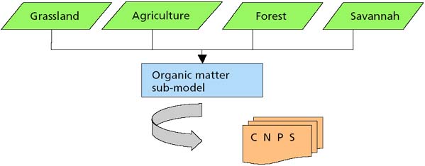
The model requires inputs of variables related to the status of C, N, P and S in the soil. The complexity and completeness of the CENTURY model is commensurate with the relatively large amounts of detailed data required to run the model of organic matter, or any of the other submodels. If the focus of study is the dynamics of C, the subset of variables required to run the model decreases in size, variables do not need to be initialized for submodels other than the SOM submodel. Information and data about all of the variables requested by CENTURY on input is not absolutely required. Data collection can be limited to only the necessary variables to obtain single carbon calculations.
As indicated earlier, the CENTURY model recognizes three types of organic materials in soils depending on their decomposition rates: resistant, slow and fast. Single calculations will require variables related to these partitions.
Information required by CENTURY per mapping unit,PCC or site
The information required by CENTURY can be divided into two types:
site characteristics data, that is, data related to the type of land mapping unit or land facet and the type of ecosystem sustained by such unit;
data on variables necessary for the parameterization of the model in the context of the particular ecosystem to be analysed.
For site variables, the information required by mapping unit, PCC or site is:
precipitation, monthly averages (from the climate station of influence);
maximum air temperature (monthly maximum temperature from the climate station of influence);
minimum air temperature (monthly minimum temperature from the climate station of influence);
content of lignin in the plant material;
content of N, P and S in the plant material;
texture of the soil;
initial contents of total S, C, N and P in the soil;
schedule of agricultural, livestock or forestry activities;
levels and amounts of agricultural inputs used during the management cycle;
production by LUT (crop yields or other units of LUT output in tonnes per hectare);
soil erosion (as soil losses in kilograms per square metre);
date of disturbances (e.g. incidence of fire, clearings or other disturbing phenomena during the study period).
Regarding specific data and information on the LUT or ecosystem under study, CENTURY models SOC on the basis of three major kinds of land use: agricultural, grassland and forest. These are selected in the model with the variable “ivauto”. Table 8 shows the codes used in CENTURY to define each of these three land-use types.
Table 9 shows the specific information needed to parameterize the model for each ecosystem or major kind of land use (as states of “ivauto”) in three columns, each containing the required information for the land-use identifier ivauto. The table is subdivided vertically in three blocks that correspond to three thematic modules of parameterization.
|
ivauto |
Major kind of land use |
|
0 |
Forest |
|
1 |
Grassland |
|
2 |
Agricultural |
|
CONCEPT |
ivauto |
||
|
|
0 |
1 |
2 |
|
Module 1 |
|
|
|
|
Bulk density |
x |
x |
x |
|
Number of soil layers or soil profile horizons |
x |
x |
x |
|
Drainage pattern |
x |
x |
x |
|
Permanent wilting point of the soil (soil moisture) |
x |
x |
x |
|
Field capacity of the soil (soil moisture) |
x |
x |
x |
|
pH |
x |
x |
x |
|
Module 2 |
|
|
|
|
Labile organic C (g/m2) |
x |
|
|
|
Non-labile organic C (g/m2) |
x |
|
|
|
C/N ratio per soil layer |
x |
x |
x |
|
Initial inputs of plant residues (g/m2) |
x |
|
|
|
C/N ratio of litter on soil |
x |
x |
x |
|
C/N ratio of the soil organic horizon |
x |
x |
x |
|
Value of the C isotope in land cover (litter) (g/cm2)1 |
x |
|
x |
|
Initial value of belowground active C2 |
x |
|
x |
|
Initial value of belowground active N3 |
x |
|
x |
|
Module 3 |
|
|
|
|
Amount of C in foliage in the forest system |
x |
|
|
|
Amount of N in foliage in the forest system |
x |
|
|
|
Amount of C in fine and coarse branches |
x |
|
|
|
Amount of N in fine and coarse branches |
x |
|
|
|
Amount of C in fine and coarse roots |
x |
|
|
|
Amount of N in fine and coarse roots |
x |
|
|
|
Initial amount of C in dead material |
x |
|
|
1 Values of DPM and RPM generated by RothC may be used as non-labile and labile C, respectively.
2 Values may be derived from data from other models (e.g. IOM, RPM and DPM of RothC-26.3, which can be identified as labile and non-labile fractions).
3 A value of N must be assigned; although this study does not require nitrogen simulation, the system models C and N simultaneously.
FIGURE 12 - Relationship between programs and file structures in the CENTURY model
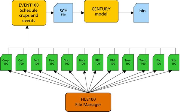
Figure 12 shows the relationship between the program modules and the file structures in the CENTURY model.
The files shown in the lower part of the chart in Figure 12 correspond to the 12 variants or components of management. Each one of these variants accounts for a large number of variables. These variant components are files within the “FILE100” structure. The large number of variables and management parameters implicit in the variants of the FILE100 structure is excessive for practical situations, particularly in conditions in the developing world. The CENTURY model may be driven by as many as nearly 650 different variables with an abundant number of variants in each of them.
It would be practically impossible to use this model if initial values for most of those parameters did not exist and had to be initialized from no values at all. In most practical situations, it is almost impossible to record so many variables in such detail. However, the CENTURY research team has generated values and tested them experimentally in a range of ecosystems. These values of parameters for the major kinds of land use (variable “ivauto”) can be used reliably as standard default values where field data are not available in any given situation. The important issue here is the good selection of the ecosystem type for which files of those standard parameters exist, and which ought to be similar or resemble the ecosystem to be modelled. The resemblance between the modelled ecosystem and the standard ecosystem files for which the model can be parameterized should be as close as possible.
It is not known with certainty, and for all situations, how robust the model is to changes in these parameters and their approximations in terms of model results with experimental data and controlled comparisons. However, the model developers (Parton et al., 1994) recommend that for reliable simulations it is best to use parameters from standard tried ecosystems suggested by the CENTURY research group, rather than to manipulate nearly 650 variables individually for which no data may be available, and for which only guesses could be made, as unpredictably wild results could be obtained in the latter situation. For example, file IRRI.100 stores four variables, the values of which have been determined through experimental analysis of several levels of irrigation (Table 10). Experimental values with different levels of irrigation have been assigned for each variable (Table 11).
|
IRRI.100 variable |
DESCRIPTION |
|
Auirri |
Controls application of automatic irrigation |
|
= 0 automatic irrigation is off |
|
|
= 1 irrigate to field capacity |
|
|
= 2 irrigate with a specified amount of water applied |
|
|
= 3 irrigate to field capacity plus PET |
|
|
Fawhc |
Fraction of available water holding capacity below which automatic irrigation will be used when auirri = 1 or 2 |
|
Irraut |
Amount of water to apply automatically when auirri = 2 (cm) |
|
Irramt |
Amount of water to apply regardless of soil water status (cm) |
|
Parameters |
A50 |
A25 |
A15 |
A75 |
A95 |
AF |
F5 |
Flood |
|
Auirri |
1.0 |
1.0 |
1.0 |
1.0 |
1.0 |
2.0 |
0.0 |
0.0 |
|
Fawhc |
0.75 |
0.25 |
0.15 |
0.75 |
0.95 |
0.25 |
0.0 |
0.0 |
|
Irraut |
0.0 |
0.0 |
0.0 |
0.0 |
0.0 |
10.0 |
0.0 |
0.0 |
|
Irramt |
0.0 |
0.0 |
0.0 |
0.0 |
0.0 |
0.0 |
5.0 |
15.0 |
Thus, when irrigation is applied at 50 percent of soil field capacity, the system will assign automatically the values corresponding to the column A50, and respectively for each level of irrigation. Because of this format, CENTURY has the possibility of being driven by nearly 650 different variables with an abundant number of variants.
The upper part of Figure 12 shows the scheduling of crops and events. These schedules require information pertaining to the SITE.100 files (site characteristics) to create a schedule file (*.sch). The schedule file is created through running the executable program “event100.exe”. Once created, this schedule file will contain all the necessary information by the model to describe crop and soil management activities for each LUT.
In order to run the CENTURY model successfully, it is necessary to generate the schedule file (*.sch) recording all management information. This in turn requires the information stored in the specific FILE100 file corresponding to the particular ecosystem that resembles the site under study. For this reason, detailed descriptions are provided below of the processes to generate both the FILE100 -including the modifications that made for modelling each site - and the schedule file through the EVENT100 routine.
Input of initial parameters through the FILE100 routine
The executable FILE100.exe is run in CENTURY as an MS-DOS command: <c:\century\file100>. A menu of options appears in the main window where the 12 types of FILE100 are listed (Figure12). On selecting one of the first 11options, the following menu appears:
What action would you like to take?
0. Return to main menu
1. Review all options
2. Add a new option
3. Change an option
4. Delete an option
5. Compare options
Enter selection:
With this menu it is possible to modify the FILE100 created by the developers of the model (University of Colorado, the United States of America), used as default for each ecosystem type. The developers do not recommend attempting to modify the default file corresponding to the ecosystem of interest in its entirety because of the hundreds of variables involved. Some of the variables required to complete the site parameterization of the model are extremely specific. In most practical circumstances, data for all such variables will not be available. Thus, the CENTURY team recommends, as the most pertinent method for entering site variables, the selection of the option (“standard” ecosystem file) that is most similar to the site to be modelled.
Returning to the initial FILE100 menu, the selection of the Site.100 option where the specific information for each site will be entered, a Site.100 file that most closely reflects the characteristics of the study site should be modified. In this option, the menu that appears is:
Which subheading do you want to work with?
0. Return to main menu
1. Climate parameters
2. Site and control parameters
3. External nutrient input parameters
4. Organic matter initial parameters
5. Forest organic matter initial parameters
6. Mineral initial parameters
7. Water initial parameters
Enter selection:
In this menu, the variables that describe the site can be input. Option 1 allows the input of data corresponding to the precipitation per month, the standard deviation of the precipitation and its skewness per month, as well as the minimum and maximum temperatures per month. Option 2 allows for the selection of site and control parameters. Here, the variable “ivauto” determines the LUT or ecosystem to be analysed. This parameter is pivotal and crucial to the choice of many other subsequent parameters. Based on its value, all other variables referred to in Module 1 (Table 9) are determined. The remaining variables retain the values in the standard Site.100 reference file.
As the objective of the methodology is the simulation of the SOC dynamics, and as the dynamic processes of C in SOM turnover are related closely to those of N, the option to simulate C and N together is justified. In CENTURY, the option to simulate only C does not exist. As far as the input of parameters of external nutrients is concerned, the variables are specific for the modelling of N and S. They should not be modified unless accurate measurements of such parameters are available, provided the default values are similar to those of the conditions of the studied site.
In Option 4, variables that are part of Module 2 (Table 9) are input. Variables in this module correspond to the specifics of C and N fractions in different morphological constituents of organic matter sources. Once these values have been input, the remaining variables are set to the default values or are assigned a value of 0, except for those that correspond to the initial N contents in the subsoil for live and inert materials. These values are assigned according to the C/N ratio of plant materials incorporated into the soil.
The variables in Module 3 (Table 9) are essentially the C and N in foliage, branches and roots. These data are input into the model in Option 5, for the simulation of forest ecosystems.
The two last options in the CENTURY menu listed above do not need to be modified. This is because the values in the standard default file containing this information satisfy the requirements of the model and its variants to obtain output values of N, P and S.
Scheduling land management options through the EVENT100 routine
The file EVENT100 was designed to include the information referring to crop and land management and other human influence on the sites being modelled. In this file, all the management activities are registered, such as the anthropogenic input of nutrients, disturbances, the specification of the periods of simulation and soil use.
The program EVENT100.exe will produce files with the extension *.sch that record the events to occur during the simulation. The schedule file becomes the basis for running the CENTURY model. Within the schedule file (*.sch), it is possible to provide detailed information to the model about the human activities that could affect the dynamics of C, such as agricultural practices and the use of chemicals, as well as the possibility of inserting the proposed standard or default variables used by the CENTURY research team, through the files Crop.100 and Tree.100. This executable program offers the possibility of changing the management regime monthly as well as by year.
The schedule (*.sch) files are created in the same subdirectory as the CENTURY model, and run with the executable program EVENT100.exe <c:\century\event100>. On execution of such command in the MS-DOS environment, the program requests the name of the FILE100 for which a schedule is to be created. The option whether or not to label C is then requested. The program also requires information as to whether or not a microcosm is to be simulated. This refers to simulation under laboratory experimental conditions. For studies on carbon stock and sequestration implicit in LUCs, it is not necessary to simulate a microcosm in lab conditions. These last two options can be set to the defaults. The user continues selecting the alternatives that reflect the conditions of the area to be evaluated, as well as the recommendation of the stochastic handling of the climate values of Site. 100.
The scheduling is set up by blocks of time (years) for which activities are planned in the DOS environment through a combination of commands (bottom row of screen) and management activities to be scheduled (left column) over the months (remaining columns) in a screen similar to that depicted in Figure 13.
FIGURE 13 - Scheduling input screen
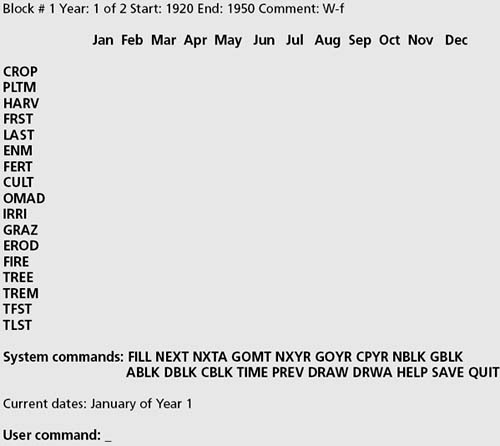
While the keys in the left-hand column refer to anthropogenic activities, the commands for manipulation of the screen are in the lower part. These are used to specify all the crop and land management activities, disturbances, as well as other events during the year or the block of time being analysed. For a full description of each of the management options listed in the left-hand column of the screen, the reader is referred to the CENTURY model operations manual. This step concludes the parameterization and data input into the model.
Running the CENTURY model
Once the site and control parameters have been input, and the crop and land management activities scheduled through the EVENT100 program, the model can be run. In the MS-DOS environment, the CENTURY subdirectory is accessed, and the model is run by providing a command which contains the name of the schedule file as well as the name of the output file on which the results of the run will be placed. This last file will have the results in binary format. The command has the following structure: <c:\century\ century -s schedule filename -n output filename> (both filenames without extension).
Given the fact that the volume of output data from the CENTURY model could be an enormous amount of information (almost 600 variables for each time block specified over the entire study period), the output is stored as a binary file (*.bin extension). The output refers to the multiple details of variables C, N, P and S. To access the results of interest to any given project, specific variables for specific years are selected from within the assembly of variables stored in the binary file. These selected variables can then be imported into spreadsheets and databases for manipulation and linkage into the GIS. The CENTURY model offers a utility for conversion from binary to ASCII formats. The LIST100 program is an executable file that creates output in ASCII format (*.lis extension) from the binary file (*.bin). The command and interactive dialogue are:
<C:\century\list100>
Enter name of binary input filename (not bin):
Enter ASCII output filename (not .lis):
Enter the starting Time, press < return > for beginning of time:
Enter ending Time, press < return > for ending time:
Enter variable, (one to per line), press < return > to enter or after blank to quit:
The variables that are deemed relevant for carbon sequestration projects are those related to the fluxes of C in soil and CO2 release. Relevant variables include: som1c(1), som2c, som3c and totc for SOC dynamics, and amt1co2, amt2co2, as11c2, as21c2, as2c2 and as3c2 for C lost to the atmosphere as CO2. The resulting ASCII file with extension “lis” contains the list of the selected variables for output. From this file, the results can be entered in a spreadsheet program and manipulated and graphed. They can also be placed in database format for linkage to GIS databases for spatial representation of results.
The case studies in this report include scenarios of carbon dynamics with different levels of inputs of crop and organic residues. These range from no management at all to realistic levels of inputs of crop residues for the areas studied. These scenarios were generated with both the RothC-26.3 and CENTURY models.
Software customization of the input/output interface of the CENTURY model -“Soil-C”
Given the complexity and the degree of difficulty involved in inputting data, creating management scenarios, parameterizing and running the CENTURY model by non-experts, it became clear that a more user-friendly graphic user interface was needed. This interface would enable non-expert users to access and run the model and to obtain useful results in situations of routine assessment of carbon stock and sequestration. During the customization of the software, it became apparent that a facility for selecting output parameters and a link to a GIS for spatial representation of modelling results were desirable.
The project generating this report undertook the customization of the CENTURY model input/output interface and GIS link. The full documentation of the customization effort can be found in Ponce-Hernandez et al. (2001). A summary description of the customization is presented in this report.
The graphical user interface (named “Soil-C”) was created as a GIS training project between Trent University and Sir Sanford Fleming College, Canada, and sponsored by FAO. Soil-C consists of a suite of programs written in Visual Basic computer language that interface with the model CENTURY (version 4.0) (available at http://www.nrel.colostate.edu/ projects/century/nrel.htm).
To run the Soil-C interface programs, it is necessary to have installed:
ESRI ArcView GIS version 3.2 or above,
Microsoft Excel (version 97 or 2000),
CENTURY (version 4.0).
The options on the main screen (Figure 14) introduce the user to a hierarchy of menus:
input site data (equivalent to input data through “FILE100”).
input management data (equivalent to input “EVENT100” parameters and creation of the schedule files).
select output variables (equivalent to choose output variables through “LIST100”).
GIS output definition.
run CENTURY.
Figures 14-19 show the initial sequence of screens for data input (Visual Basic forms). The CD-ROM accompanying this report contains a demo of the Soil-C interface program, the Soil-C program and the user manual.
The experience gained by running the model for the generation of several land-use scenarios through case studies was an important factor in the decision to customize the interface to the CENTURY model. It is believed that users of the model can save considerably on learning time by using the interface, provided the results they need are simple enough to be within the capabilities included in the customization.
FIGURE 14 Initial screen of the Soil-C interface
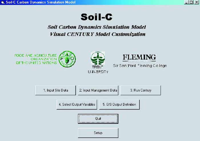
FIGURE 15 Input of site parameters in the Soil-C interface
FIGURE 16 Input of site parameters: climate variables in Soil-C
FIGURE 17 Organic matter initial parameters for specific ecosystems
FIGURE 18 Scheduling events and management with the Soil-C interface
FIGURE 19 Selection of output variables and output file specification for interface with GIS
![]()
![]()
![]()
)
)
)
)
)