Macrolevel

This study calculated the macrolevel nutrient balance on a grid basis. As land use is the main driver of the nutrient flows and balance, it formed the basis for the methodology. A procedure exists to create a land-use map, based on suitabilities, and showing the most likely crop distribution. This study combined the grid map (cell size of 1 km) with other spatial data that were necessary for the nutrient-balance calculation. As exported to MS Access, the resulting attribute table contained all the spatially explicit data: livestock densities, soil, rainfall, Harmattan dust, erosion-sedimentation and irrigated areas. The program MS Access performed the calculation of the soil nutrient balance and the results were exported to ArcView. The final outcomes require aggregation where the intention is to use them for display purposes because a 1-km grid is too detailed for the macrolevel. Where possible, all input data were averaged for the years 1997 - 99.

Land-use map

It is not possible to link land cover data as retrieved from satellite images to management data because land cover does not describe crop distribution. On the other hand, it is not possible to link national statistics, as provided by the FAOSTAT database, to climate and soil data because the spatial distribution is unknown. The methodology described below generates land-use maps for any given African country on the basis of available data sets. The basis of the proposed methodology lies in the traditional qualitative land evaluation, where land qualities are matched with land-use requirements in order to find the suitability of land for different uses (FAO, 1976). The methodology for land-use mapping comprises three key steps:

Step 1: Identify land units with similar topography, climate and soil conditions.
Step 2: Match properties of the land units with crop requirements.
Step 3: Disaggregate harvested areas from FAOSTAT over the land units.

Step 1

The first step identifies land units defined by topography, soil and climate. Topography is described by a global 30-arc second digital elevation model (DEM) GTOPO30 (USGS, 1998). The 1:5 000 000 FAO soil map of the world describes the soils (FAO/UNESCO, 1997). However, the legend of the soil map indicates the soil classification and does not provide quantitative estimates of soil properties. Batjes (2002) developed the world inventory of soil emission potentials (WISE) database that provides quantitative estimates of soil properties for all the soil classes of the FAO soil map of the world. For climate, this study used the global climate database compiled by the International Institute for Applied Systems Analysis (IIASA), as developed by Leemans and Cramer (1991). The global AEZs (FAO and IIASA, 2000) provided information about the length of the growing period as a function of weather conditions. However, such an evaluation is only useful where the area is actually being cropped or grazed. The United States Geological Survey (USGS), the University of Nebraska-Lincoln (the United States of America), and the European Commission’s Joint Research Centre have carried out a global land cover assessment using two subsequent satellite images (USGS et al., 2000). This study used the ‘seasonal land cover region’ legend, reclassified into eight main classes. All areas under agriculture were reclassified as cropland or mixed cropland/natural vegetation.

The maps were projected using a Lambert azimuthal equal-area projection with a central meridian at 20° and a reference latitude of 5°. The next step was to convert the maps to a 1-km grid (where necessary) before overlaying them onto a single 1-km grid. These maps contained data on altitude, soils, climate, growing period and land cover. By linking the databases it was possible to create a table with the following land characteristics: land cover, length of growing period, rainfall, temperature, soil depth, texture, drainage and altitude.

Step 2

The second step includes the traditional matching process, as per the FAO qualitative land evaluation system (FAO, 1976), which compares land qualities with crop requirements. However, lack of available data at this scale level did not allow for an assessment of land qualities. Therefore, the available land characteristics as listed above formed the basis for the evaluation. The crop environment response database ECOCROP (FAO, 1998a) describes crop requirements, expressed in the same way as land characteristics. ECOCROP provides information on crop requirements for 1 710 different crops, grasses and trees. For many crop requirements, the database provides minimum and maximum values as well as optimal ranges.

A program developed in Delphi matches the land units with the 32 main crops and fallow described in the FAOSTAT database through the respective land characteristics and crop requirements. The result of the matching process is a six-digit code that represents the classification of the six key land characteristics from 1 (not suitable) to 3 (suitable) as illustrated in Figure 8. The code lists the land characteristics in sequence from highly important (left) to less important (right). Thus, it is possible to sort the suitability codes and obtain an automatic ranking of the likelihood of finding a specific form of land use on the land unit.

Step 3

The final step of the procedure is to allocate the crops according to the suitability classification. The FAOSTAT database provided the actual areas of each crop. This database contains national data on the harvested areas for the most important agricultural crops. A predefined crop order file determines the order in which crops are allocated. This study ranked crops mainly on the basis of their economic importance (Table 8), i.e. it allocated an important cash crop such as tea to the most suitable locations and a less important food crop such as millet to less suitable places. Each crop is distributed to the areas with the highest suitability for that specific crop, unless other crops already fill the area. This means that crops that are high in the crop order are allocated to the most suitable places. An exception was fallow, because fallow depends not on suitabilities but on the character of a particular land-use system. Therefore, the fallow area was split and allocated by ratio to those crops related with fallow systems, which are mainly cereals and root crops. This adaptation delivered a more realistic pattern for the fallow areas, where fallow is located in the same area as the crops of that particular land-use system. It was not possible to simulate directly short-distance variation in cropping systems or multiple cropping. This is because only one land use can be allocated to each grid cell. However, by aggregating the final results to a larger grid size, these systems were taken into account indirectly. It was possible to link the resulting output table of the simulation to the original grid map, and the land-use map showed the most likely distribution of crops, based on suitabilities.

TABLE 8
Crop order for the land-use-map procedure

Model parameters

IN1: Mineral fertilizer

The input of mineral fertilizer was calculated per crop. Each crop was given a fraction of the total fertilizer nutrient consumption. The fractions were based on data of the fertilizer-use-per-crop studies of the International Fertilizer Industry Association (IFA), the International Fertilizer Development Center (IFDC) and FAO (IFA/IFDC/FAO, 2000). These data were not available for every country. For Ghana and Mali, this study used data from surrounding countries within the same AEZ. The total fertilizer consumption per country was taken from the FAOSTAT database. The program MS Access then calculated the average amount of fertilizer per crop in terms of kilograms per hectare.

Example calculation

For a ‘maize’ grid cell in Kenya, the calculations were:

TABLE 9
Number of animals per country

Source: FAOSTAT.

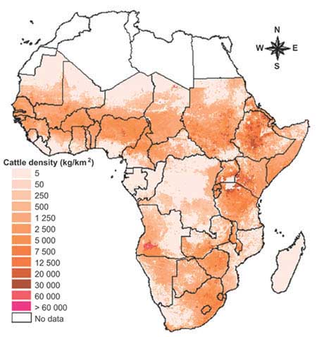
IN2: Organic inputs

Livestock density maps developed by FAO and the environmental research group of Oxford Limited (Figure 9) (FAO, 2000) were available for the major livestock classes, i.e. cattle, small ruminants and poultry (Table 9). The poultry density map was based on the rural population of SSA (FAO, 2001b). The number of poultry was presumed to have the same spatial distribution as the rural population. The livestock densities were multiplied by the excretion per animal per year (Table 10) and the nutrient content of the manure (Table 11). This generated the total amount of nutrients produced per livestock class. Annex 9 gives the literature sources for the nutrient values used.

TABLE 10
Excretion

Source: Derived from Fernandez-Rivera et al. (1995).

TABLE 11
Nutrient content of manure (fresh weight)

Source: Derived from sources in Annex A.

Although the total amount of nutrients produced by livestock is known, the losses and their distribution remain undetermined. According to Fernandez-Riviera et al. (1995) and Schlecht et al. (1995), animals produce 43 percent of their manure at night in their stable/corral/boma. Thus, 57 percent of the manure, losses excluded, remains in the field (grid cell). The other 43 percent, losses excluded, might be relocated to specific crops and fields. Moreover, such a study as the present one should consider livestock from grid cells without crops. This is because livestock relocates nutrients from pastureland to the stable and afterwards to the crops. Therefore, the livestock density maps were aggregated to a 30-km grid, which represents the average manure availability in a region. This average amount was multiplied by an aggregation factor and a crop factor. The aggregation factor was country dependent and related to the population density. This factor was 2 for Ghana and Mali, and 1.5 for Kenya, because of the greater population density. The crop factor determines whether a specific crop receives manure (1), twice as much manure (2), or no manure (0). Annex 7 presents the estimates of these factors for each country.

During grazing, manure is lost along roadsides and other places where no crops are growing. These losses were estimated at 15 percent for all countries. The losses during storage are probably larger because manure also has other uses, such as fuel and house construction material. Losses also occur during storage and manifest themselves through leaching, denitrification and volatilization. A factor for such losses depends considerably on the type of management, and different factors were used for each country. The estimated losses for Ghana, Mali and Kenya were 40, 25 and 15 percent, respectively. These percentages were based on population density, livestock system and the relative importance of manure as a fertilizer. Manure is not collected as intensively in Ghana as in Kenya because livestock is not as important and the population density is lower. Kenya has more ‘semi-grazing’ and ‘zero-grazing’ systems, while Ghana and Mali have mainly ‘free range’ systems. For the calculated manure application, the losses due to leaching, denitrification and volatilization were calculated in OUT3 and OUT4.

Summary of calculation procedure per grid cell

This calculation was performed for each livestock group (cattle, small ruminants and poultry) and these values were summed.

Example calculation

For a ‘maize’ grid cell in Kenya and a cattle density of 100 kg/ha (about 50/km²) the calculations were:

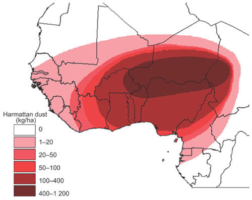
IN3: Wet and dry deposition

The input of nutrients by deposition consists of two parts: wet deposition related to rainfall; and dry deposition related to Harmattan dust. Factors for nutrient contents were calculated based on literature values (Tables 12 and 13). A map with Harmattan dust deposition values was created by interpolation, based on several literature sources (Table 14) and wind-stream patterns (Pye, 1987; McTainsh, 1980; McTainsh and Walker, 1982; Kalu, 1979). Figure 10 provides the details. The amount of dust was derived from this map, whereas the amount of precipitation was derived from the IIASA rainfall map (Leemans and Cramer, 1991).

Example calculation

For a grid cell in Ghana with 1 200 mm of rainfall and 80 kg of Harmattan dust per hectare, the calculations were:

TABLE 12
Nutrient content of rainwater

TABLE 13
Nutrient content of Harmattan dust

TABLE 14
Amount of Harmattan dust at various locations

IN4: N fixation

Input by BNF consists of different parts, i.e. symbiotic N fixation by leguminous crops, non-symbiotic N fixation and N-fixing trees. From the literature (Giller, 2001; Danso, 1992; Giller and Wilson, 1991; Hartemink, 2001), the percentages of total N uptake derived from symbiotic N fixation were:

Groundnut - 65 percent;
Soybean - 67 percent;
Pulses - 55 percent;
Sugar cane - 17 percent.

For wetland rice, cyanobacteria fix N, and this study used a value of 15 kg N/ha per year. This value is somewhat lower than that estimated in many experiments but according to Giller (2001) the effect of the cyanobacteria is overestimated and it does not occur in all fields. This N fixation occurs only in wetland rice, but in Africa more than 50 percent of the rice area is upland rice. However, FAOSTAT does not differentiate between wetland and upland rice. Therefore, the amount of N fixation by cyanobacteria was multiplied by a factor for wetland rice. According to Nyanteng (1986) and the IPCC (1997), Ghana has 15 percent wetland rice, Kenya 25 percent and Mali 95 percent. Not much literature is available for nonsymbiotic N fixation and N-fixing trees. This input was estimated on the basis of the amount of rainfall using the following equation (N fixed is expressed in kg N/ha and rainfall in mm/year):

N fixed = 0.5 + 0.1 × Ö rainfall

Example calculation

For a ‘groundnut’ grid cell in Ghana with a rainfall of 1 000 mm and a yield of 1.2 tonnes/ha, the calculation was:

IN5: Sedimentation

This flow consists of two parts: nutrient input in irrigation water; and input in sediment as a result of erosion. FAO and the University of Kassel, Germany, have developed a worldwide map of irrigation areas (Döll and Siebert, 2000). The nutrient input was calculated by combining this map with the estimated amount of irrigation water, set at 300 mm/ha/year, and the nutrient content of irrigation water (N: 3.3 mg/litre, P: 0.43 mg/litre and K: 1.4 mg/litre) derived from Stoorvogel and Smaling (1990). The input by sedimentation was calculated by the “LandscApe ProcesS modelling at mUltidimensions and Scales” (LAPSUS) model (Schoorl et al., 2000; Schoorl et al., 2002), which also provided a feedback between IN5 and OUT5. Details are given under OUT5. The model output was the net sedimentation in metres. It was possible to convert this value into nutrient input by combining it with bulk density and nutrient content.

Example calculation:

For an ‘irrigated rice’ grid cell in Mali, in the absence of sedimentation, the calculations were:

OUT1: Crop products

This study calculated the output of nutrients by crop products by multiplying yield by the nutrient content of the crops (Table 15). FAO statistics (FAOSTAT) provided data on harvested area, production and, hence, yield for each country.

Example calculation

For a ‘maize’ grid cell in Kenya, the calculations were:

OUT2: Crop residues

This study calculated the output of nutrients in crop residues by multiplying crop residue yield by its nutrient content (Table 15) and adjusting this by a removal factor. The latter is crop and country specific, is based on scarce literature values and expert knowledge, and reflects the type of management. Removal factors for central Kenya, with a high population density and many animals, are larger than those for southern Ghana, where livestock are relatively unimportant. A special form of residue removal is ‘burning’, but it is difficult to determine its extent at the macrolevel. Therefore, burning was considered solely for cotton, because farmers normally burn these residues in order to prevent pests and diseases. All N is lost by volatilization and an estimated 50 percent of all K is lost directly through leaching.

TABLE 15
Nutrient content of harvested product, crop residues, and removal factors for crop residues

Example calculation

For a ‘maize’ grid cell in Kenya, the calculations were:

OUT3: Leaching

Leaching can be an important outflow for N and K. De Willigen (2000) developed a regression model to estimate the amount of leached N. This model is based on an extensive literature search and is valid for a wide range of soils and climates. A new regression model for K leaching was developed, based on the same data set:

The N-leaching regression model is based on 43 different measurements and accounts for 67 percent of the variance (De Willigen, 2000). The equation was edited slightly for perennial crops by multiplying the amount of N in soil organic matter by 0.5. This prevented overestimation of N leaching, because perennials can take up N throughout the year. The K-leaching regression model is based on 33 representative experiments and has an R2 value of 0.45 (Annex 2 for references).

Example calculation

For a ‘maize’ grid cell on a ferric Luvisol in Kenya, with a yield of 1.8 tonnes/ha and a fertilizer application of 50 kg N/ha and 30 kg K/ha, the calculations were:

OUT4: Gaseous losses

Two processes cause the bulk of gaseous N emissions: denitrification and volatilization. Denitrification takes place under anaerobic conditions but soil does not have to be fully saturated for denitrification to occur. A moist soil loses nitrates through microbial processes in wet films and pockets. The expectation is for losses through denitrification to be greatest in wet climates, on highly fertilized and clayey soils. Ammonia (NH₃) volatilization plays a role mainly in alkaline soils, but such soils are not very common at the macrolevel in SSA. Therefore, volatilization and denitrification in soils do not receive separate treatment. Volatilization is also linked directly to the amount of mineral and organic fertilizer.

This study developed a regression model to estimate gaseous N losses. The equation consisted of two parts: one regression model for the N₂O and NO_x losses through denitrification, and a direct loss factor for volatilization of NH₃. The equations were based on literature data for tropical environments (Annex 4). These were derived from a larger data set compiled for a recent study to estimate global gaseous emissions of NH₃, NO and N₂O from agricultural land (IFA/FAO, 2001). The N₂O regression model was based on a data set of 80 experiments and had an R² value of 0.45. The NO_x regression model was based on 36 different measurements and had an R² value of 0.91. For NH₃ emissions, 73 measurements were available. Of all fertilizer N applied, 11.3 percent is lost, with a standard deviation of 6.2 percent.

Example calculation

For a ‘maize’ grid cell with a ferric Luvisol in Kenya, with a mineral and organic fertilizer application of 50 kg N/ha, the calculation was:

OUT5: Erosion

Erosion is difficult to estimate, yet it can be important. To estimate erosion, this study utilized the LAPSUS model. This model simulates the amount of erosion and sedimentation at the landscape scale. This method has several advantages: it generates quantitative data; it considers erosion at the landscape scale; and it takes sedimentation into account. This is preferable to literature estimates, because the latter rely mainly on plot experiments, which are not representative for the macrolevel.

Basic concepts

This study used a modelling approach based on work by Kirkby (1971; 1978; 1986) and Foster and Meyer (1972; 1975). They assume the potential energy content of flowing water over the landscape surface as the driving force for sediment transport. Another important assumption is the use of the continuity equation for sediment movement. This states that the difference between sediment input and output equalizes the net increase in storage. Assuming quasi-steady state, Foster and Meyer (1972; 1975) formulated down-slope sediment transport continuity as:

where z is elevation (m), t stands for time, C is sediment transport capacity (m²/ time), and S is the sediment transport rate (m²/time). Term h stands for detachment rate under erosion conditions, while it represents the settlement rate under sedimentation conditions. To estimate the change in elevation dz over time step dt, it is necessary to calculate the changes in the sediment transport rate dS. These changes in the rate of transport are controlled by the transport capacity C, where the capacity excess will be filled by detachment of sediment (e.g. erosion, surface lower), and a capacity deficit will lower the amount of sediment in transport (e.g. sedimentation, surface higher). According to Foster and Meyer (1972; 1975), after integration, assuming that transport capacity and detachment or settlement capacity remain constant within one finite element, the calculation for the rate of sediment in transport is:

S = C + (S₀ - C) · e^-dx/h

where the transport rate S (m²/time) over the length dx of a finite element is calculated as a function of transport capacity C (m²/time) and detachment rate or settlement rate h compared with the amount of sediment already in transport S₀ (m²/time). S is expressed as soil volume per unit grid width per year. To convert to erosion or deposition rate in mass per area per year, S is divided by the grid length (dx) and multiplied by soil bulk density. Term h (m) refers to the transport capacity divided by the detachment capacity (m/time) (C/D) or to the transport capacity in proportion to the settlement capacity (-m/time) (C/T). Implementation of this equation will need expressions for transport capacity C, detachment capacity D and settlement capacity T. These capacities are calculated as functions of discharge and slope, which gives:

C = a · Q^m · Lⁿ

where C is calculated as a function of discharge Q (m²/time) and slope tangent (dz/dx) L [-], m and n are constants (dummy variable a corrects the units). Assuming, inter alia, that detachment and settlement capacity are proportional to a certain shear and that the drag coefficient is constant, the equations are:

D = K_es · Q · L
T = P_es · Q · L

where K_es is a lumped surface factor (per metre) indicating the erodibility of the surface and P_es a similar factor indicating lumped sedimentation characteristics (per metre). The erosion conditions for D or sedimentation conditions for T will result in opposite signs for the change in S and as a result also dz.

Model structure and flow routing

LAPSUS is based on a grid structure of square cells of equal size. Each cell presents a generalized part of the landscape that can comprise several unique characteristics (altitude, soils, etc.). The model is structured in a way that is optimal for the simulation of both two-dimensional and three-dimensional characteristics in the time dimension. In this way, the model considers the evaluation of capacities as a two-dimensional process because only the gravitational force and water flow downslope within a finite element are used. However, for the estimation and routing of the incoming and outgoing water and sediment fluxes, the model evaluates the results of surrounding grid cells within the whole three-dimensional landscape. The finite element methodology implies variable length but a unit width at different resolutions for each element.

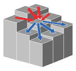
Landscape process modelling

The LAPSUS model evaluates the rates of sediment transport by calculating the transport capacity of water flowing downslope from one grid cell to another as a function of the discharge and the gradient of the slope. A surplus of the transport capacity of the water is filled by the detachment of sediment, which depends on the erodibility, K_es (per metre), of the surface. This detachment of sediment provokes lowering of the surface or erosion. However, when the rate of sediment in transport exceeds the local capacity, e.g. because of lower gradients, a settlement function will deposit the surplus of sediment in transport, thereby causing a higher surface or sedimentation. The routing of the overland flow and the resulting model calculations are done with a multiple flow algorithm in order to enable a better representation of divergent properties of the convex topography (Figure 11). The modelling framework underwent elaborate testing for the effects of changing flow algorithms, spatial resolution and temporal resolution. LAPSUS has only been validated for its base scenario by field observations in southern Spain, but it displays erosion and sedimentation patterns which match closely with real world erosion and sedimentation patterns at the same spatial resolution.

The main input parameters for the grid-based LAPSUS model are the topographical potentials (slope gradients) from a DEM and the evaluation of the rainfall surplus that will generate the overland flow. The assumption is one of uniform conditions for all involved parameters within each grid cell. The model will evaluate all considered parameters on an annual basis for a certain run of time. Other input parameters are soil depth, to estimate the amount of infiltration, and erodibility (K_es). It is possible to determine these parameters from a geology or soil map. Moreover, a land use or land cover map can serve as input for the estimation of the amount of runoff. The LAPSUS model can now run for the chosen number of years and input parameters.

The present study used the following input data:

DEM with a resolution of 1 km (USGS, 1998);
land cover map (USGS et al., 2000);
rainfall map (Leemans and Cramer, 1991) and data for Kenya (Corbett and White, 1998);
soil erodibility (K factor), derived from soil map of the world (FAO/UNESCO, 1997);
soil depth, derived from soil map of the world (FAO/UNESCO, 1997).

Annex 5 describes the exact procedure and factors used for the model.

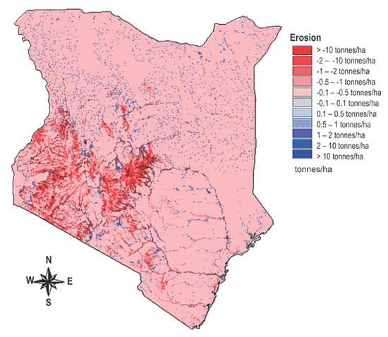
The outcome of the model is a net erosion-sedimentation map with units in metres, convertible to tonnes per hectare (Figure 12). It is possible to calculate the loss or gain of nutrients by multiplying by soil nutrient contents and an enrichment factor. The enrichment factor reflects the fact that the finer and more nutrient-rich soil particles will be dislodged earlier during erosion. Based on literature data, the study used the following enrichment factors: 2.3 for N, 2.8 for P, and 3.2 for K (FAO, 1984; FAO, 1986 and Khisa et al., 2002). It is possible to derive the nutrient content of the soil from the soil map. As a result of erosion, the rooting depth zone is extended, which means that new nutrients come within reach of plant roots. This study assumed that 25 percent of P and K, which is lost due to erosion, was gained at the rooting zone through this process.

Example calculation

For a grid cell on a ferric luvisol in Kenya, with 1 mm erosion, the calculations were:

Fallow

The FAO statistics did not provide details on the area under fallow. However, it was possible to calculate it indirectly by subtracting the total sum of harvested areas from the total arable land (Table 16). IN1 and OUT1 are not relevant for fallow. IN2 and OUT2 are related as they comprise grazing animals and the same defecating animals. It is not known whether IN2 should be larger or smaller than OUT2. Not all manure is left on the field (only about 57 percent), but on the other hand a lot of animal feedstuff is obtained from sources other than crop residues, and from roadside grazing. Hence, for fallow land the amount of nutrient input by manure (IN2) was presumed to be equal to the amount lost by grazing (OUT2). All other nutrient flows can be treated equally as for other crops.

TABLE 16
Fallow area for Ghana, Kenya and Mali

Source: Derived from FAOSTAT.