CHAPTER 1 - FROST PROBABILITY AND RISK OF DAMAGE

Importance of probability and risk

The most effective methods of frost protection are to plant crops that are not sensitive to freezing, plant in locations without freezing temperatures, or plant a crop that emerges or blooms after the danger of frost has passed. The first two methods are rarely achievable if you want to produce a particular product in a site that has freezing temperatures. In most areas of the world outside of regions with only tropical climates, subzero temperature is possible. Even in countries with tropical climates, frost events can occur at high elevations. The probability and risk of damaging temperatures changes with time of the year and, for some crops, sensitivity to damaging subzero temperatures also changes. Knowing the probability and risk is important because it helps growers to decide whether, what and when to plant at a particular location. The probability gives you the 'odds' that you will experience damaging temperature in any given year and the risk tells you the probability that this is likely to occur over a design period (e.g. the expected life in years of a tree crop or a frost protection method). Therefore, frost probability and risk analysis is a useful decision-making tool.

Making decisions about frost protection depends on the type of crop to be grown. For example, frost can damage annual 'field and row' crops and the probability of frost damage is mainly affected by plant selection for winter crops and when you sow for spring-planted crops. For winter crops, the damage will often occur in the coldest part of the winter. Using probability and risk calculations, one can determine the odds that the crop is damaged by frost. If the risk is high, the winter cereal could be replaced with a spring cereal to reduce losses. Haan (1979) presented the methodology to determine the probability and risk for crops that are commonly damaged by severe freezes in midwinter. He showed how to calculate the probability that temperature will fall below a critical damage temperature in any given year and he showed how to determine the risk of this happening one or more times over a given number of years. The approach is similar to that used by hydrologists when determining flood return periods or geologists estimating the probability and risk of earthquakes. Probability and risk statistics for floods and earthquakes are used to make decisions about how much money to invest in buildings and structures to avoid damage and loss of life.

Similarly, probability and risk information on minimum temperatures is used to make decisions about the odds that a crop will be lost to frost damage in any given year or over several years. The odds are then used to decide if the crop should be planted, if it is worthwhile to invest in insurance, if a different crop should be planted, or if frost protection is cost-effective.

Knowing the exact probability of reaching a specified critical damage temperature on any given date in the spring and autumn is useful for determining annual crop plant and harvest dates and the desirable length of growing season to avoid frost damage. The procedure to estimate these probabilities and an Excel application program 'FriskS.xls' to make the calculations is provided with this book.

For fruit trees and vines, the critical damage temperatures change with developmental stage of the crop and the dates of the growth stages vary from year-to-year. Consequently, determining probability and risk for orchard and vine crops is more complicated than for annual crops. For example, a critical damage temperature (T_c) might be -7 °C or lower at early bud break but it can increase to -2 °C or higher during small fruit stage a month or so later. An application program (TempRisk.xls) is provided with this book to calculate the probability and risk associated with a critical damage temperature during a specified period of time corresponding to a growth stage. For example, the T_c and beginning and ending dates for the period of interest are input into the application. Then, using 20 years or more of minimum temperature climate data, the probability that the temperature will fall below T_c during that period in any given year and the risk that it will happen one or more times within 5, 10,..., 30 years are computed and graphically displayed. The calculation methods and instructions to use the TempRisk.xls are discussed in this chapter.

Risk and certainty calculations

Risk analysis is used to estimate the chances that a damaging event will or will not occur in the long term (i.e. over several years). For example, a grower wants to know the risk that a particular crop will be lost to frost over the expected lifetime of the crop or the design life for a frost protection method. In this book, the risk is determined using a method presented by Haan (1979) using a binomial distribution (i.e. a Bernoulli process). In a binomial distribution, the risk (R) of having one or more occurrences of temperature below the selected minimum temperature over a period of n years is calculated as:

where = = 1.C is the combination of n things taken 0 at a time and P⁰ = 1.0.

Simplifying this expression gives the equation:

where P = P (T < T_c). Since this is the risk of having one or more damaging frost events within n years, the certainty (C) of having no frost events is given by:

Therefore, the probability (P) of having a frost event within any given year can be calculated from the certainty (C) as:

where C is the fractional probability that the event will not occur within a specified number of years (n). A table of one-year event probabilities corresponding to a range of certainty and design periods (years) is given in Table 1.1. For example, to be 90 percent certain (i.e. C = 0.90) that the minimum temperature will not fall below a particular damaging temperature (T_c) within the next 15 years, the probability that this event will occur in any given year must be less than 0.007 or 0.7 percent (i.e. in 1 000 years, it should not happen more than seven times).

TABLE 1.1

Probability (P) of an event occurring in any given year corresponding to the certainty (%) that the event will not occur during the design period

Event probability calculations

Recall in the previous section that a probability P = 0.007 corresponded to a 90 percent certainty that an extreme event would occur in no more than 7 years of 1 000 years. The probability of an extreme event happening in any given year would ideally be determined by calculating the ratio of the observed extreme events over the number of years of record. However, typically one is fortunate to have 20 or 30 years of data, rather than the 1 000 or more years needed. Since data are limiting, the best approach is to determine a probability density function from the existing data set. The probability density function is an approximation for what is expected if a 1 000 or more years of data were available. There are many types of probability density functions, but Haan (1979) reported good results for minimum temperature data using a type I extreme value probability density function. The cumulative curve for a type I extreme value probability density function is:

where a = s/283, b = m + 0.45a, m is the mean minimum temperature and a is the standard deviation of the minimum temperatures over the years of record. Therefore, by calculating the mean and standard deviation of the minimum temperatures over years, calculating a and b and inserting them into Equation 1.5, one can find the probability that the minimum temperature in any given year will fall below T_c. The resulting probability (P) of the event occurring within any given year can be input into Equation 1.3 with the design period (n) to estimate the certainty that an extreme temperature below T_c will not occur within the n years. For example, if P = 0.0111 and the design period is 20 years, this corresponds to C = 80 percent certainty that the event will not occur within a 20-year period (Table 1.1).

Crops with fixed sensitivity

Haan (1979) presented a method to estimate probability and risk of temperature falling below a critical value when the sensitivity of the crop to damage is fixed. The model was modified and an MS Excel application program ‘TempRisk.xls' was written to make the calculations for a user-selected time period. Probabilities are calculated using a type I extreme value function and the risk is calculated using a Bernoulli process. The TempRisk.xls application program is included with this book.

Data entry

Up to 50 years of minimum temperature data can be input into the 'Data' worksheet of TempRisk.xls (Figure 1.1) and analysed to calculate the probability and risk. More accuracy is associated with more years of data, but a minimum of 20 years of data are required for reliable analysis. The beginning and ending dates for the time period being evaluated and the critical temperature are input in cells in the upper left of the 'Data' worksheet and the probability of exceeding the event is displayed below the critical temperature cell.

Probability output

The probability of the minimum temperature falling below the critical temperature within the period in any given year is displayed on the 'Data' worksheet. However, the probability of having a lower temperature for a range of subzero temperature is plotted in the 'FrostProb' chart (Figure 1.2). For example, from Figure 1.2, there is about an 8 percent probability that the minimum temperature will fall below -4 °C during the period 1 May through 20 December for the data that were entered into TempRisk.xls.

Risk worksheet and chart

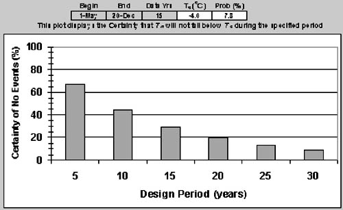
The certainty of having no minimum temperature below the critical damage temperature for design periods of 5, 10,..., 30 years are plotted in the 'Risk' chart of TempRisk.xls (Figure 1.3). For example, there is about 65 percent certainty that the minimum temperature will not fall below -4 °C within a 5-year period. At the same time, there is only about 10 percent certainty that this will not occur during a 30-year period. Clearly, a longer design period has more chances for damage to occur.

FIGURE 1.1

A sample of the 'Data' worksheet for the TempRisk.xls application program

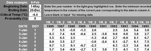
FIGURE 1.2

The probability of having a lower minimum temperature during a specified time period (from the 'FrostProb' chart of the TempRisk.xls application program) plotted against the corresponding minimum temperature

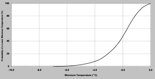
FIGURE 1.3

Certainty (%) of no events with the minimum temperature falling below the input critical temperature (i.e. -4.0 °C) between 1 May and 20 December within a 5, 10,..., 30-year design life (from the 'Risk' worksheet and chart of the TempRisk.xls application program)

Last spring and first autumn frost dates

Knowing the probability associated with the last damaging frost date in the spring and the first damaging frost date in the autumn are important for planning when to plant a crop. For example, a later planting date is appropriate if the probability of damaging temperature is too high in the spring. If the probability of damaging temperature is high before harvest in the autumn, then planting a shorter season variety is wise. It is also advantageous to know the probability and risk when evolving longer-term strategies for planting and harvesting dates, and for variety selection. In addition to identifying possible frost problems, analysing probability and risk provides information on the odds that these problems will occur. Therefore, it is useful to decide an acceptable level of risk for growing a crop as well as for deciding if frost protection is justifiable. The application program FriskS.xls is provided with this book to make the probability and risk calculations associated with the last spring and first autumn frost dates.

Data entry

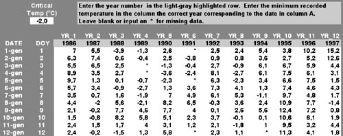
The accuracy of probability calculations from temperature data is limited by the years of data, so a greater number of years gives a more accurate estimate. To use the FriskS.xls application, input a minimum of 20 years of daily minimum temperature data into the Data worksheet. However, use more years of data if available. It is important to put the year corresponding to the temperature data at the top of the data column. A critical temperature is input in a cell near the top left hand side of the Data worksheet (Figure 1.4).

FIGURE 1.4

A sample of data input into the Data worksheet of the FriskS.xls application program, with a critical temperature T_c = 0.0 °C

Probability output

After data entry, FriskS.xls calculates the probabilities that a minimum temperature below the input critical temperature will occur on a date later in the spring. Similarly, the probabilities that a minimum temperature below the input critical temperature will occur on a date earlier in the autumn are computed. Then the probabilities for having a minimum temperature lower than the input critical temperature on a date later in the springtime or earlier Z in the autumn is plotted versus date in the 'FrostProb' chart (Figure 1.5).

Growing-season chart

The FriskS.xls application also calculates probabilities for the length of growing season. Here the length of the growing season is defined as number of days between the mean last date with a minimum temperature below the input critical temperature in the spring and the mean first date with a minimum temperature below the input critical temperature in the autumn. The probabilities are plotted versus date in the 'GrowingSeason' chart. An example is shown in Figure 1.6.

Risk worksheet and chart

The certainty of having no dates after a selected date in the spring with a minimum temperature below the critical temperature (e.g. T_c = 0.0 °C) is calculated and displayed in the 'SpringRisk' worksheet and chart (Figure 1.7). The selected date (i.e. to determine the probability that T < T_c on a later date) is input at the top of the SpringRisk worksheet (e.g. 20 March in Figure 1.7). The probability (%) that a day with T < T_c will occur after that date in any given year is calculated and displayed. Then the certainties (%) that no temperature below T_c will be observed during a 5, 10,..., 30-year design period are displayed as a column graph. For example, there is about 45 percent certainty that no temperature below T_c = 0 °C will be observed after 20 March, but there is less than 1 percent certainty that no temperature below 0 °C will occur after 20 March during a 30 year period (Figure 1.7).

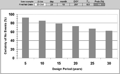
A similar procedure is used to calculate and display certainties that a minimum temperature will fall below T_c before a selected date in the autumn. Figure 1.8 shows a sample from the 'FallRisk' worksheet with a selected date of 1 November and a T_c = 0.0 °C. The certainties are again displayed as a column graph. For example, there is close to 85 percent certainty that there will be no minimum temperatures below 0 °C before 1 November during a 5-year period. For a 30-year period, the certainty is only about 35 percent.

FIGURE 1.5

A plot of the probability of having a date with the minimum temperature lower later in the spring or earlier in the autumn versus date (from the FrostProb chart of the FriskS.xls application program)

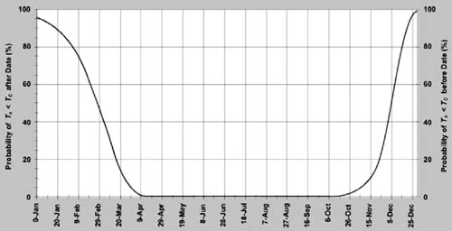
FIGURE 1.6

Probability of fewer days between the last date in the spring and the first date in the autumn with minimum temperature below the input critical temperature (from the 'GrowingSeason' chart of the FriskS.xls application program)

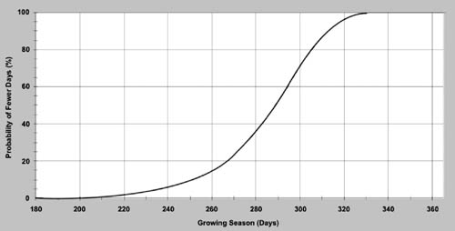
FIGURE 1.7

Certainty (%) of no events of the minimum temperature falling below the input T_c after '20 March' over 5, 10,..., 30 years (from the 'SpringRisk' worksheet and chart of the FriskS.xls application program)

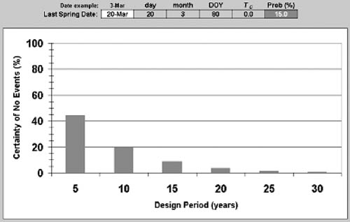
FIGURE 1.8

Certainty (%) of no events of the minimum temperature falling below T_c before 1 November over 5, 10,..., 30 years (from the 'FallRisk' worksheet and chart of the FriskS.xls application program)

Calculation methods

The FriskS.xls application program first determines the last spring date when the minimum temperature falls below the input critical temperature for each year. Then it calculates the mean (m_d) and standard deviation (s_d) of the last spring date over the years of record. The probabilities for the last spring date are calculated using:

where 'd' is the day of the year, a_d =s_d/1.283 and b_d = m_d + 0.45a_d.

For the first date of damaging temperature in the autumn, the mean and standard deviation of the first date in the autumn is computed over the years of record and the probabilities are calculated using the same equations for a_d, b_d and P(T_n < T). The certainty calculations for the SpringRisk and FallRisk charts are done using Equation 1.3. For the growing season calculations, the yearly difference between the last spring date and the first autumn date are used to compute the mean and standard deviation over years. Then the same equations used for the last spring and first autumn dates are used to calculate the probabilities of having fewer days in the growing season.

Damage Estimator (DEST.xls) application

The MS Excel Damage Estimator application program - DEST.xls - is used to calculate expected frost damage and crop yield using site-specific maximum and minimum temperature climate data for crops having no protection against frost, and using up to 11 different frost protection methods. Up to 50 years of maximum and minimum temperature data can be used in the analysis. Critical temperatures associated with 90 percent (T₉₀) and 10 percent (T₁₀) damage are input corresponding to specific phenological dates. Frost damage is assumed to be multiplicative. For example a frost causing 50 percent damage followed by a second event of 50 percent damage will result in a 75 percent yield loss (i.e. 50 percent in the first event and 50 percent of 50 percent = 25 percent in the second event). It is assumed that damage is directly related to the minimum temperature and it is unrelated to the duration at a minimum temperature.

The program is structured into three steps. In the first step, the estimated °C of protection expected for the 11 protection methods are input into the 'Start here' worksheet (Figure 1.9). Then input the crop name, crop height, n plants per hectare, type of plant and expected yield without frost damage. If the crop is thinned, input the percentage of fruit to remove in the appropriate cell. If the crop is not thinned, leave 0 percent in the thinning cell. When rerunning the application, type 'Y' in the "Erase all previous inputs" cell to remove earlier entries. Leave in 'N' or type 'N' to leave the entries shown in the worksheet. When finished with entries, click on 'Complete Step 1 of 3' to continue to Step 2.

FIGURE 1.9

Sample entries for the 'Start here' worksheet

In the second step, input the maximum and minimum temperature climate data. An example of the first few days of several years of maximum and minimum temperature data is shown in Figure 1.10. It is only necessary to enter data for the period when frost damage is likely to occur. This period should bracket the dates when critical temperatures exist in the table included in the "Crop" worksheet. When finished, click on 'Complete Step 2 of 3' to continue.

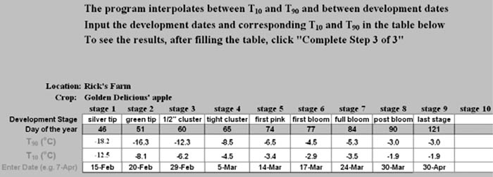
Finally, the third step is to input the critical temperature data corresponding to dates of sensitive phenological stages. For example, Figure 1.11 shows the entry of T₉₀ and T₁₀ data and dates for phenological stages of apple cv. Golden Delicious. The program will only analyse the data between the first and last date with critical stages. Therefore, a "last stage" entry should be made as shown in Figure 1.11 so the last period is identified.

FIGURE 1.10

A sample of entry of maximum and minimum temperature for the 'Weather' worksheet

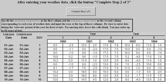
FIGURE 1.11

Sample entry of T₉₀ and T₁₀ data corresponding to the dates of critical phenological stages into the 'Crop' worksheet

When finished with the 'Crop' worksheet, click on 'Complete Step 3 of 3' and the application displays the output in the RESULTS worksheet where you will find:

1. A table of yearly percentage frost damage to the fruit or nut set for an unprotected crop and the 11 protection methods (Figure 1.12)

2. A table of yearly yield on a tonnes per hectare basis for the unprotected crop and the 11 protection methods. If a percentage of the fruit or nut thinning was input into the 'Start here' worksheet, there is no yield reduction until that percentage of fruit or nut set is lost to frost damage first. Thus, if there is a frost event, it is assumed that the frost damage thinned the crop and only losses in addition to the thinning will affect final yield.

3. A summary table with yearly averages and standard deviations of percentage losses of the fruit or nut set and means and standard deviations of crop yields (Figure 1.12).

4. The mean and standard deviation of the number of frost events and the duration of the frost events are shown in a summary table.

FIGURE 1.12

A sample of the 'RESULTS' worksheet showing the means and standard deviations of percentage damage and yield for the 11 protection methods and for no protection

The worksheet also shows the fraction of potential yield lost to frost damage and the expected marketable yield by year and protection method. In the DEST.xls application, the bottom table is displayed to the right of the middle table.

Calculation of the physical risk of frost damage was investigated in this chapter, and use and interpretation of the physical risk damage calculator (DEST.xls) was presented. In the next chapter, the financial decision of whether or not to implement frost protection is investigated, and evaluated in economic terms. The concept of risk is therefore extended from physical risk to financial risk. A personal computer program is presented to support decision-making.