![]()
![]()
![]()
To estimate fish production and yield using the analytical approach, fundamental studies are undertaken on growth and the natural mortality rates (death of fish due to causes other than fishing) of fish.
Growth of fish is the change in body weight over time and is the difference between anabolism (building-up of body substances) and catabolism(breaking down of body substances). This can be written as:
| dw/dt= | HWd-kw | (Pauly 1984) | |
| where: | dw/dt= | change in body weight per unit time | |
| H= | coefficient of anabolism | ||
| k= | coefficient of catabolism | ||
| W= | weight of the fish | ||
When the above equation is integrated and weights are replaced by length, the equation gives the widely known model - the Von Bertalanffy Growth Formula (VBGF):
| Lt | = L∞ (1-exp(k(t - to))) | |
| where: | Lt | = length of fish at time t |
| L∞ | = asymptotic length i.e. the mean length a given stock would reach if they were to grow indefinitely | |
| K | = growth constant | |
| to | = age of fish at time zero | |
| t | = time (years) |
The parameters L∞ and K are of paramount importance in management of any fishery using analytical approach. These are used in models such as the Beverton and Holt Yield Per Recruit Model which are used to manage a fishery.
It should be noted here that L∞ and K are dependent of each other. Often fish which have high values of L∞ have low corresponding values of K and vice versa. Therefore, these values can not be used to compare performance of stocks. To compare performance of the stocks, a growth performance index known as the phi-prime (Æ) based on both L∞ and K is often used. In this study, growth performance index (Æ) was estimated according to Vakily (1988):
Æ = log K + 2 * log L∞
While fish grow and therefore lead to increase in fish biomass growth, there are opposite tendencies which lead to biomass decrease. Such tendencies are the death of fish. Over time fish die due to either natural mortality M or due to fishing mortality F. The natural and fishing mortality rates add up to total mortality rate. The number of fish in a stock is presented as:
| Nt | = No.exp(-Zt) | |
| where: | Nt | = number of fish that remain at the end of time t |
| No | = initial number of fish | |
| Z | = instantaneous rate of total mortality, which is the sum of F and M |
Various methods are used to estimate growth parameters. L∞ and K: those that are based on length of fish, some on catch data and others on tag-recapture experiments. With catch numbers of fish at two different times using the same effort, mortality rates can be estimated.
Length-based methods were used to estimate growth parameters and population estimates of fish.
When length frequency of fish is plotted over time one can follow the growth of fish by following up the modes (mode is the number with the highest frequency of occurrence). A growth curve can be fitted to progression of such modes either by “paper and pencil” or by using a computer. The ELEFAN method is one of the computer-based methods.
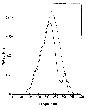
The Compleat ELEFAN Software package of Ganayilo et al (1989) was used to analyse growth of O. shiranus based on length-frequency (L/F) data obtained from catches by gill nets. Gill net are well known for high values of selectivity. To adjust the samples for selectivity, selectivity factors from a study by Mattson (1994) from Mbvoniha were used. These were obtained from combined selectivity (of meshes between 16.5 to 43 mm) (Figure 1). Few fish were caught in meshes lower than 16.5 mm (Mattson, pers.comm.). Since selectivity values were available for fish of length group between 70 and 80 mm and above, adjustments were made on classes of this length group and above. Although selectivity study was conducted on Mbvoniha, it was found that the selectivity values were applicable for Mikolongwe (Mattson 1994).
Adjusted catch data were analysed by small water body and sex using the Compleat ELEFAN. The procedure used involved the following steps:
smoothing of the L/F data, through a running average of 5 (classes) using ELEFAN 0 to reduce variability due to low sample sizes;
estimation of L∞, and estimation of the other parameters of the VBGF modified for seasonal growth i.e. K (year-1), C, expressing the amplitude of seasonal growth oscillations (0<C>1) and the Winter Point (WP) expressing the time of the year (as a decimal fraction) when growth is slowest (Gayanilo et al. 1989). This was done using various routines of ELEFAN I program.
Catch (in numbers) at each time by gill nets was adjusted to remove bias due to selectivity as outline in section 3.1.1. Total mortality coefficient Z between two different times was estimated by:
| Z = 1/t2-t1 * ln N(t2)/N(t2) | (Sparre et al, 1989) |
Natural mortality (M) was estimated using empirical relationship of Pauly (1980, as quoted by Arias-Gonzalez et al 1993), i.e:
log10M = 0.0066 - 0.279log10L∞ + 0.6543log10K + 0.4634 log10T
| where: | L∞ = asymptotic length in cm; |
| T = the mean environmental temperature in degrees C; | |
| K = growth constant | |
| Since: | Z = F + M |
| where: | F = fishing mortality |
The fishing mortality can be defined as:
F = Z - M
Figure 1: Combined selectivity curve for multimesh gillnet meshes 16.5 to 43 mm (bar height) (----- = Model selectivity, = raw data.). From Maltson (1994)
A computer based Virtual Population Analysis (VPA) method was used to estimate fish production. “Virtual” means what was actually fished in terms of number of fish. The method is incorporated in ELEFAN III program.
The VPA estimates the number of fish which were in the small water body to account for the catch. In this method length frequency data were converted to catch and biomass at length when:
biomass of each catch from which the length-frequency data were obtained was estimated;
the length-weight relationship for the sexes and species in the different small water bodies was used:
W = aLb
Which was transformed to:
log W = log a + b log L
| where: | W = weight of fish in grams |
| L = total length of fish in cm |
The catch-at-length data were used to estimate the fishing mortality for each size class. The natural mortality and fishing mortality which were estimated in 3.1.2 were used in the VPA. The value of fishing mortality was used as the Terminal Fishing mortality rate (Ft).
With tagging, it was possible to estimate the growth of individual fish when the fish was recaptured interval after a certain time. The Gulland and Holt plot, using length and age data, can be used to estimate the growth parameters.
Fish of different lengths (ages) were marked, and intervals between tagging and recaptured were different. To obtain estimated growth parameters, fish were put into groups according to their lengths at tagging. The length groups were 0–10, 10–13, 13–15, 15–17, 17–20, and >20 cm. Since fish growth rates differ according to age, and growth according to logistic curve was assumed, for length groups of below 15 cm only those which were recaptured within 100 days, were included in the analysis. It was assumed that growth of fish in this category would have a different growth rate after 100 days. Following the same rationale, for fish groups which were above 15 cm only those which were recaptured within 200 days were included in the analysis. Growth parameters L∞ and K were estimated using the Gulland and Holt plot of the form:
dL/dt = K. (L∞ - L(t))
Which can be written as:
| dL/dt = KL∞ - kL(t) | (Sparre et al 1989) |
and if in the equation,
KL∞ = a and K = b
Regression dL/dt over KL(t) gives intercept a and regression coefficient b. Note that L(t) is the mean length of fish during the corresponding period of length increment dL/dt. The parameters K and L∞ were obtained from:
K = -b
where: L∞ = -a/b.
Mortality rates for the tag-recapture methods were reflected in the survival rates estimated together with the population estimates. Population estimates for each sampling date were made according to the Seber-Jolly method (Ricker 1975). Following notation from Ricker (1975), “C”, M, m, k and R were estimated “Ci” was the number of fish examined for tags at ith sampling. Since fish of 10 cm and above were tagged, all fish which were caught using gill nets and were above 10 cm (including those which were tagged) plus recaptures from either seine nets or gillnets in total were the “C”. Mi was the total number of fish tagged at time i; ki was the sum of all recaptures made later than Time i of fish tagged before Time i. Rij are recaptures of fish tagged at Time i and recaptured at the next marking (j). R12 are recaptures of fish tagged at Time 1 and recaptured the second tagging. R23 were fish tagged at the second tagging (in this case, month “2”) and recaptured at month “3”. An example of the estimation of the parameters is given in Table 3:
Table 3: The Seber-Jolly (Ricker 1975) estimates for Mikolongwe
| Date | Fish newly marked (Mi) | Fish examined for marks (Ci) | Markings at different months | |||||||||
| 1 | 2 | 3 | 4 | 5 | 6 | 7 | 8 | m | k | |||
| 10/2/93 | M1=877 | |||||||||||
| 10/5/93 | M2=301 | C2=631 | R12=49 | m2=49 | k2=97 | |||||||
| 29/6/93 | M3=164 | C3=391 | R13=39 | R23=11 | m3=50 | k3=100 | ||||||
| 3/8/93 | M4=149 | C4=316 | R14=16 | R24=10 | R34=19 | m4=45 | k4=105 | |||||
| 15/9/93 | M5=131 | C5=278 | R15=21 | R25=16 | R35=18 | R45=11 | m5=49 | k5=63 | ||||
| 27/10/93 | M6=121 | C6=254 | R16=16 | R26=10 | R36=2 | R46=8 | R56=13 | m6=66 | k6=35 | |||
| 9/12/93 | M7=52 | C7=134 | R17=5 | R27=4 | R37=7 | R47=3 | R57=7 | R67=6 | m7=32 | k7=12 | ||
| 9/1/94 | M8=149 | C8=220 | R18=0 | R28=2 | R38=4 | R48=2 | R58=1 | R68=2 | R78=3 | m8=49 | k8=1 | |
| 2/3/94 | C9=156 | R19=0 | R29=0 | R39=0 | R49=0 | R59=0 | R69=1 | R79=0 | R89=1 | m9=2 | ||
Where:
k2 = R13+R14+R15+R16+R17+R18+R19
k3 = R14+R15+R16+R17+R18+R19+R24+R25+R26 R27+R28+R29
k4 = R15+R16+R17+R18+R19+R25+R26+R27+R28+R29+R35+R36+R37+R38+R39
k5 = R16+R17+R18+R19+R26+R27+R28+R29+R36+R37+R38+R39+R46+R47+R48+R49
k6 = R17+R18+R19+R27+R28+R29+R37+R38+R39+R47+R48+R49+R57+R58+R59
k7 = R18+R19+R28+R29+R38+R39+R48+R49+R58+R59+R68+R69
k8 = R19+R29+R39+R49+R59+R69+R79
After estimations of Mi, Ki, and Ri were made, Bi (the number of tagged fish in the population just before the ith sampling) and Nt (total number of fish per time) were estimated by:
Bi = (Mi *Ki/Ri) + mi
and:
| Nt = Bi*Ci/mi | (Ricker 1975) |
Survival rates (Si) of fish from Time i to Time i + 1 were estimated by:
Si = Bi+1/Bi-mi + Mi
Si is the probability of survival of an individual from one end of the ith sampling to the beginning of the i +1th sampling (Jones 1977).
Empirical models were used to estimate fish yields and production in the two small water bodies. Five models based on total phosphorus(TP), transparency, and the morpho-edaphic index (MEI) were used.
Based on total phosphorus (TP)
| (1) | Log Y = 0.708 log TP + 0.774 | (Hanson and Leggett, 1982) |
| (2) | Log Y = 0.072 TP+0.792 | (Hanson and Leggett, 1982) |
Based on transparency
| (3) | Y = 229(±128) + 32974(±8788)/Transparency | (Moreau and De Silva, 1991) |
Based on the Morphoedaphic index (MEI)
The yield was estimated based on the Morphoedaphic index (MEI):
| MEI = Kz-1 | (Cochrane and Robarts 1986) |
| where: | K = conductivity, | |
| z = mean depth (m) | ||
| (4) | Y = 14.314 MEI0.4681 | (Henderson & Welcomme (1974, as quoted by Moreau and De Silva 1991) |
| (5) | Y = 23.281 MEI0.447 | (Marshall 1984 as quoted by Cocharane and Robarts 1986) |
![]()
![]()
![]()