![]()
![]()
![]()
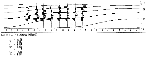
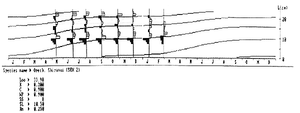
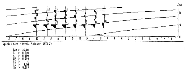
Table 4 shows L∞, K, C and WP for different sexes and reservoirs with Rn values which are indices of goodness of fit in the ELEFAN program. The Rn values show how good the growth curve fits the data. The values range between 0 and 1. The higher the value, the better the fit is. Adjusted length frequency data with superimposed growth curves are presented in Figures 2 – 5.
Mikolongwe SEX1
Figure 2: Restructured length frequency (L/F) data as used by ELEFAN I, program to fit a seasonalised oscillating, growth curve of male O.Shiranus in Mikolongwe
Mikolongwe SEX 2
Figure 3: Restructured length frequency (L/F) data as used by ELEFAN I, program to fit a seasonalised oscillating, growth curve of female, O. Shiranus in Mikolongwe
Mbvoniha SEX 1
Figure 4: Restructured length frequency (L/H), data as used by ELEFAN I, program to fit a seasonalised Oscillating, growth curve of male, O. Shiranus in Mbvoniha
Mbvoniha SEX 2
Figure 5: Restructured length frequency (L/F) data as used in ELEFAN I program to fit a seasonalised oscillating growth curve of female, O. Shiranus in Mbvoniha
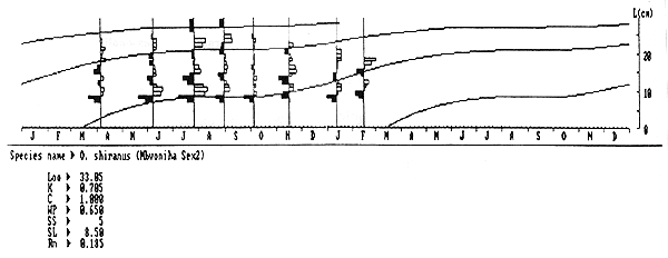
Table 4: Growth parameters of fish from different sexes and water bodies as estimated using ELEFAN 1.
| Growth parameter | Mikolongwe | Mikolongwe | Mbvoniha | Mbvoniha |
| Male | Female | Male | Female | |
| L∞ | 31.5 | 33.90 | 35.6 | 33.05 |
| K | 0.35 | 0.30 | 0.31 | 0.71 |
| C | 0.81 | 0.90 | 0.10 | 1.00 |
| WP | 0.91 | 0.90 | 0.69 | 0.65 |
| Rn | 0.211 | 0.250 | 0.189 | 0.185 |
| Æ | 2.54 | 2.51 | 2.59 | 2.89 |
L∞ and K estimated Table 4 were reasonable. The values of index of goodness fit (Rn) were almost the same (although slightly higher for Mikolongwe than Mbvoniha), but generally were low. Such low values suggested that there were recruitment pulses.
In Table 5, comparison of growth parameters is made between results from this study and those from Domasi experimental station (in the same region) where the parameters were estimated in similar way (although on mixed sex).
Table 5: Comparison of growth parameters of O. shiranus from Mikolongwe/Mbvoniha and the Domasi experimental station.
| Growth parameter | Mikolongwe | Mbvoniha | Data from the station* | ||||
| male | female | male | female | Pond 1 | Pond 2 | Pond 3 | |
| L∞ | 31.5 | 33.9 | 35.6 | 33.05 | 27.3 | 18.0 | 15.3 |
| K | 0.35 | 0.30 | 0.31 | 0.71 | 0.51 | 0.91 | 1.71 |
| Æ | 2.54 | 2.51 | 2.59 | 2.89 | 2.58 | 2.47 | 2.60 |
Results from Table 5 show that although the L∞ and K values from the station were lower and higher (respectively) than those from Mikolongwe and Mbvoniha, Æ values were almost the same.
With tag-recapture data, the growth parameters estimated using the Gulland and Holt plot are presented in Table 6.
Table 6: Growth parameters for different sexes and small water bodies from tag-recapture data estimated using the Gulland and Holt plot.
| Growth parameter | Mikolongwe | Mbvoniha) | ||
| Male | Female | Male | Female | |
| b | -0.271 | -0.32 | -1.5744 | -0.832 |
| a | 11.147 | 10.332 | 41.386 | 25.46 |
| R squared | 0.523 | 0.782 | 0.9759 | 0.9335 |
| Calculated L∞ | 41.13 | 32.29 | 26.29 | 30.60 |
| K | 0.271 | 0.32 | 1.57 | 0.832 |
| Æ | 2.66 | 2.50 | 3.04 | 2.89 |
Results in Table 6 show that L∞ and K values were higher and lower (respectively) in Mikolongwe than in Mbvoniha. However, the Æ values were lower in Mikolongwe than in Mbvoniha.
Growth parameters from length frequency and tag-recapture analysis on different sexes and small water bodies are compared in Table 7.
Table 7. Growth parameters from length frequency and tag recapture in Mikolongwe and Mbvoniha
| Method of Analysis | Mikolongwe | Mbvoniha | ||||||||||
| Male | Female | Male | Female | |||||||||
| L∞ | K | Æ | L∞ | K | Æ | L∞ | K | Æ | L∞ | K | Æ | |
| Length frequency | 31.5 | 0.35 | 2.54 | 33.9 | 0.30 | 2.51 | 35.6 | 0.31 | 2.59 | 33.1 | 0.7 | 2.89 |
| Tag-recapture | 41.1 | 0.27 | 2.66 | 32.3 | 0.32 | 2.50 | 26.3 | 1.57 | 3.04 | 30.6 | 0.8 | 2.89 |
Results in Table 7 show that with the two methods of analysis differences in Æ values only occurred in male fish of Mbvoniha. The rest Æ values were almost the same.
Estimates of population (number of fish) for each size class, mortality (instantaneous) and exploitation rates (see Figures 6 to 9 in appendix II) and steady state biomass from the length frequency data using the VPA (Virtual Population Analysis ref. Page 10, point 3.1.3) method incorporated in ELEFAN III are presented in Tables 8 and Table 9.
Table 8: Estimates of population for different length classes, mortality and exploitation rates and biomass of different sexes in Mikolongwe using Virtual Population Analysis
| Length class (cm) | Catches (N) (Male) | Population estimates (Male) | Catches (N) (female) | Population estimates (female) |
| 7.00–8.00 | 165864 | 357168 | 195128 | 530909 |
| 8.00–9.00 | 68881 | 190006 | 83868 | 299877 |
| 9.00–10.00 | 50241 | 120345 | 47651 | 193599 |
| 10.00–11.00 | 12141 | 69608 | 11229 | 130578 |
| 11.00–12.00 | 5045 | 57113 | 20359 | 107465 |
| 12.00–13.00 | 11217 | 51748 | 14165 | 77514 |
| 13.00–14.00 | 12222 | 40248 | 15167 | 56096 |
| 14.00–15.00 | 10917 | 27806 | 11361 | 35741 |
| 15.00–16.00 | 4163 | 16738 | 5224 | 21029 |
| 16.00–17.00 | 2558 | 12468 | 2277 | 13631 |
| 17.00–18.00 | 2789 | 9823 | 1997 | 9791 |
| 18.00–19.00 | 2041 | 6965 | 4193 | 6635 |
| 19.00–20.00 | 1563 | 4871 | 1182 | 1869 |
| 20.00–21.00 | 1465 | 3268 | 243 | 516 |
| 21.00–22.00 | 867 | 1777 | 56 | 213 |
| 22.00–23.00 | 422 | 895 | 53 | 125 |
| 23.00–24.00 | 315 | 465 | 26 | 55 |
| 24.00–25.00 | 142 | 146 | ||
| Total mortality (Z) | 3.31 | 1.853 | ||
| Fishing mortality (F) | 3.27 | 1.15 | ||
| Exploitation rate (E) | 0.988 | 0.621 | ||
| Steady state biomass (tonnes) | 136.18 (54.6 t/ha) | 186.39 (74.6 t/ha) |
Table 9: Estimates of population for different length classes, mortality and exploitation rates and biomass of different sexes in Mbvoniha using Virtual Population Analysis
| Length class (cm) | Catches (N) (Male) | Population estimates (Male) | Catches (N) (female) | Population estimates (female) |
| 7.00 – 8.00 | 78858 | 391176 | 92835 | 308414 |
| 8.00 – 9.00 | 22853 | 275179 | 46036 | 198144 |
| 9.00 – 10.00 | 15428 | 22980 | 23318 | 139923 |
| 10.00 – 11.00 | 6388 | 182406 | 15204 | 107278 |
| 11.00 – 12.00 | 8473 | 153972 | 10795 | 84508 |
| 12.00 – 13.00 | 2977 | 126081 | 10529 | 67438 |
| 13.00 – 14.00 | 6462 | 105993 | 8631 | 51756 |
| 14.00 – 15.00 | 5187 | 84569 | 9833 | 39003 |
| 15.00 – 16.00 | 4977 | 66665 | 6634 | 26076 |
| 16.00 – 17.00 | 4588 | 51042 | 4491 | 17265 |
| 17.00 – 18.00 | 4915 | 37765 | 1787 | 11257 |
| 18.00 – 19.00 | 3120 | 26062 | 1158 | 8350 |
| 19.00 – 20.00 | 2145 | 17812 | 767 | 6298 |
| 20.00 – 21.00 | 1104 | 11824 | 787 | 4803 |
| 21.00 – 22.00 | 1084 | 7849 | 603 | 3435 |
| 22.00 – 23.00 | 5867 | 4689 | 112 | 2386 |
| 23.00 – 24.00 | 681 | 2683 | 168 | 1911 |
| 24.00 – 25.00 | 280 | 1145 | 0 | 1432 |
| 25.00 – 26.00 | 0 | 431 | 0 | 1161 |
| 26.00 – 27.00 | 84 | 194 | 0 | 916 |
| 27.00 – 28.00 | 154 | 697 | ||
| 28.00 – 29.00 | 142 | 375 | ||
| Total Mortality Z | 1.298 | 5.121 | ||
| Fishing mortality F | 0.565 | 0.961 | ||
| Exploitation rate E | 0.435 | 0.759 | ||
| Steady state biomass(tonnes) | 231 (77 t/ha) | 311 (104 t/ha) |
Results in Table 8 and 9 show that both for small water bodies female fish were in higher abundance than the male fish at the beginning of the study period, however the fishing pressure was higher for male than female fish in Mikolongwe while for Mbvoniha it was the opposite: it was higher for female than the male fish.
Estimates of population numbers from tag-recapture study using the Jolly-Seber method are presented in Table 10.
Table 10: Population estimates (numbers) and survival rates estimated using the Jolly and Seber method
| Month, Year (Sampling day) | Mikolongwe | Mbvoniha | ||||
| April, 1993 | Nt | Twt(kg) | S | Nt | Twt(kg) | S |
| - | - | - | 1633 | 91.4 | 0.70 | |
| May | 727 | 36.4 | 0.44 | - | - | - |
| June | 956 | 47.8 | 1.41 | 3582 | 200.59 | 0.63 |
| July | 4894 | 244.7 | 0.57 | 1581 | 88.5 | 0.68 |
| September | 1933 | 96.6 | 0.99 | 804 | 45.02 | 2.90 |
| October | 2690 | 134.5 | 0.81 | 2822 | 158.03 | 0.26 |
| December | 1005 | 50.2 | 0.62 | - | - | - |
| January 1994 | 2561 | 128.05 | - | 683 | 38.2 | 0.75 |
| February | - | - | 2072 | 116 | - | |
Note:
Twt = Total weight
Average weight of fish for Mikolongwe = 50 grams
Average weight of fish for Mbvoniha = 56 grams
Results in Table 10 suggest that the highest number of fish in Mikolongwe was in the month of May and for Mbvoniha it was in June. Fish biomass ranged between 36.4 kg to 244 kg for Mikolongwe and between 45.02 kg to 200.59 kg for Mbvoniha. It should be noted that survival rates higher than one were reported for both Mikolongwe (June) and Mbvoniha (July).
Estimation of yield based on the empirical prediction gave the following results:
| Small Water Body | Area | Mean Depth | Conductivity | MEI (based on conductivity) | Total Phosphorus | Transparency |
|---|---|---|---|---|---|---|
| Mikolongwe | 2.5 ha | 3.5 m | 167 uS/cm | 47.7 | 0.013 mg/1 | 41 cm |
| Mbvoniha | 3 ha | 2.5 m | 364 uS/cm | 145.6 | 0.05 mg/1 | 43 cm |
Table 11: Estimated yield and production in both Mbvoniha and Mikolongwe based on empirical methods using morphoedaphics, physical and chemical characteristics
| Model | Estimated yield (kg/ha/year) | Estimated yield (kg/year) | |||
| Mbvoniha | Mikolongwe | Difference (%) | Mbvoniha | Mikolongwe | |
| 1 | 0.78 | 0.27 | 35 | 2.3 | 0.68 |
| 2 | 6.25 | 6.21 | 99 | 18.75 | 15.53 |
| 3 | 995.8 | 1033 | 103 | 2985 | 2582.5 |
| 4 | 147 | 87 | 59 | 441 | 217.5 |
| 5 | 215 | 131 | 60 | 645 | 327.5 |
Table 11 shows that different models gave different yields in the two small water bodies. The production figures from Mikolongwe were 35 per cent lower than Mbvoniha using Model 1, but were almost the same for both small water bodies using models 2 and 3. Using models 4 and 5, yields from Mikolongwe were 60 per cent lower than those of Mbvoniha. Models 4 and 5 were used at other places in Malawi (Brooks 1993) and results are compared to those from this study in the Table 12.
Table 12: Estimated yields from Mikolongwe and Mbvoniha and from a mean of eleven small water bodies in the north of Malawi using models 4 and 5
| Model | Mikolongwe (kg/ha/yr) | Mbvoniha (kg/ha/yr) | Average for 11 small water bodies (kg/ha/yr)* |
| 4 | 87 | 147 | 67 |
| 5 | 131 | 215 | 101 |
* Data from Brooks 1993 (unpub.)
As can be noted from Table 12, using the same models, production estimated for Mikolongwe and Mbvoniha were higher than for most small water bodies in the northern region of Malawi.
The yield/production and biomass estimates using the different analytical methods used in this study are presented in Table 13.
Table 13: Yield/production and biomass estimates in Mikolongwe and Mbvoniha using length frequency, tag recapture and empirical methods.
| LENGTH FREQUENCY DATA Biomass at the beginning of experiment (kg/ha) | TAG RECAPTURE METHOD Average biomass during experiment (kg/ha) | EMPIRICAL METHOD Fish production kg/ha/month (average of 5 models) | |
| Mikolongwe | 129028 | 42.2 | 20.9 |
| Mbvoniha | 180763 | 35.1 (1293*) | 22.7 |
* From Mattson (1994) (single catch tag-recapture method was used)
Table 13 shows that estimates using length frequency were more than the estimates using the other two methods. Empirical methods estimated lowest production from the small water bodies. Single catch tag-recapture method (Mattson 1994) gave higher biomass estimates than the multiple catch tag-recapture method used in this study.
Inputs required to collect data for the different analytical methods: length frequency, multiple catch tag-recapture and catch recording of catch data are presented in Table 14.
Table 14: Inputs required to collect data for different methods of analysis.
| Tag-recapture (multiple) | Length -frequency | Catch data | |
| Equipment | Tags | Measuring board | Weighing balance |
| Personnel per sampling | 3 1- for recording 2- for tagging | 2 1-for measuring 1- for recording | |
| Time spent each at sampling | 10 hrs (tagging 100 fish) (fish have to be carefully handled so that they are returned alive) | 3 hrs (measuring 100 fish) | |
| Other personnel requirement | 1 (for the whole study period to record any tags reported by fishermen) | 1 (for the whole study period to record catches by fishermen) | |
| Total labour input (manhours) to run a study for one year with sampling every month | 9120 | 72 | 8760 |
![]()
![]()
![]()