![]()
![]()
![]()
As previously mentioned, the work is divided in two main sections for presentation purposes. The first section (3.1) deals with the analysis of the climate regimes and their possible connections to interdecadal ENSO variability. The second section (3.2) is dedicated to the definition and analysis of small pelagic regimes. Finally, an integrated view of the relation between climate and small pelagic regimes is attempted.
3.1.1. Identification of global climate regimes
3.1.2. Global climate regimes as reflected by wide-coverage air temperature series
3.1.3. Climate regimes and El Niño relative strength and frequency
3.1.4. Climate regimes as reflected by the SOI index
3.1.5. Decadal scale El Niño relative strength and frequency and the SOI
In this section, results of the analysis of the global climate regimes are presented and discussed. First, we show that climate regimes are detectable as the interdecadal variability of the GSAT series. Regime periods, as identified within this series, are compared to decadal signals of other large-coverage air temperature series. Finally, the same periods are used to show variations of the frequency and relative strength of ENSO events and of the long-term trends within the SOI.
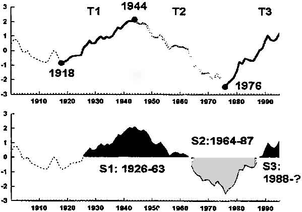
Figure 3 shows the detrended and smoothed GSAT series. Sustained warm-cold periods, sustained long-term trends, and wide fluctuations are evident only during the final part of the series (P2, solid line). Before 1918 (PI, broken line) the variability is lower, as no value reaches one standard deviation positive nor negative. Cooling-warming trends and cold-warm periods are shorter that those after 1918, which may indicate that before this year the global climate variability was dominated by phenomena of a shorter frequency than regime changes (at least, shorter than the documented regimes of abundance fluctuations of sardine and anchovy). Given that small pelagic regimes are only documented for the present century, we decided to focus only on the second period (P2). This is not to say that possible relationships between interdecade variability, ENSO variations, and small pelagic abundances do not exist before 1918, but the current lack of evidence of small pelagic fluctuations makes it difficult to evaluate them for those early years.
Figure 3. Detrended, smoothed (simple exponential transformation), and standardized GSAT series.
After 1918, three sustained long-term trends are evident from the transformed series (see Figure 4). The first is a 27 year upward-trend that lasted until 1944, which happens to be the year with the highest positive difference from the long-term trend line. Then, a sustained downward trend took place until 1976, the year with the largest negative deviation. Finally another upward trend goes to at least 1995. Between these long term trends, sustained periods of positive (warm) and negative (cold) anomalies are also evident. From 1926 until 1963 values are positive, the period between 1946 and 1987 is one of negative values, and since 1988 values have been positive again.
Tables 1 and 2 show these periods and trends together with the abundance fluctuations of the main sardine and anchovy stocks. Broadly, it can be noted the warming trends have coincided to periods when sardine (anchovy) abundance increases (decreases), and the warm periods include several years of high (low) sardine (anchovy) abundance. Similarly, cooling trends generally coincide with increasing (decreasing) anchovy (sardine) abundance, and cool periods include several years with large (small) anchovy (sardine) population levels. This scheme is particularly evident for the California area, and generally applicable to the Japan and Humboldt Systems. Allowing for the opposite species arrangement, the Benguela sardine is also in general agreement with the mentioned scheme, and only the Benguela anchovy seems to behave in a different and unique way.
Table 1. Regime-related periods and trends and abundance variability of the main sardine stocks. Abundance trends as described by Lluch-Belda et al. (1992), except: (I): All years above 100 MT except 1953, according to data from Barnes et al 1992. (2) See Smith 1990. (3) See Barnes et al. 1992. (4) Implies biomass in excess of 18,000 MT.
|
Period |
California |
Japan |
Humboldt |
|
1918-44 |
Catch increased (1916-36) |
Catch increased (1915-36) |
No data until early 1970s, since a significative fishery started after the collapse of the anchovy stock. |
|
1926-63 |
High catches during the 30s and 40s. High spawning biomass off California up to 1960 (1) |
High catches from mid 1920's to mid 1940's, but decreasing since late 1930's. |
|
|
1944-76 |
Catch decreased (1945-60). Spawning biomass off California decreased rapidly on 1941-53 (2). |
Already scarce, remained low until 1975. |
|
|
1964-87 |
Low catches since 1952 Spawning biomass remained low during 1966-86 (2). |
|
|
|
1976-onwards |
Increasing trend of sardine biomass since late 1970s (3). |
Catch increased during 1975-88. |
Catches increased (1977-1988), and spawning biomass since 1974 until 1982. |
|
1988-onwards |
Direct fishery allowed since 1986 (4). |
High catches during 1981-91, but decreasing since 1989. |
High catches (1984-1991), but decreasing since then. |
Table 2. Regime-related periods and trends and abundance variability of the main anchovy stocks. Regime-related periods and trends and abundance variability of the main sardine stocks. Abundance trends as described by Lluch-Belda et al. (1992), except: California biomass data kindly provided by A. MacCall for SCOR WG98. (2) South Africa biomass data kindly provided by R. Crawford for SCOR WG98.
|
Period |
California |
Japan |
Humboldt |
|
1918-44 |
No data available |
Low catches until late 1950's, with no evident sustained trend. |
No data available |
|
1926-63 |
|
|
|
|
1944-76 |
Biomass rapidly increased on 1969-74. |
Catches increased during 1946-56. |
Catches increased during 1960-1970 |
|
1964-87 |
High biomass during 1974-86. High catches until 1989. |
High catches during 1954-72. |
High catches during 1962-71. |
|
1976-onwards |
Biomass decreasing since 1976, catch decreasing since 1981. |
Catches decreased during 1973-89. |
Catches decreased during 1972-84. Lowest catches during 1977-85 |
|
1988-onwards |
Biomass lowest values since 1989. |
Low catches during 1977-89, increased for 1990. |
Rapidly increasing since 1986 |
For the identified climate regime trends and periods, it is important to establish whether these are earth-scale signals or just regional phenomena. The fact that regimes are evident from the GSAT series cannot be considered as definitive evidence, because this series averages all the available observations, thus implying very different spatial and temporal coverages. The ideal way to establish the spatial coverage of the regime signal would be to analyze temperature series from small areas, but only a few can be calculated back in time to make the analysis possible. Therefore, the use of series averaged for large areas is usually the only possibility for building time series long enough to reflect regime variations.
Figure 5. Detrended, smoothed (simple exponential transformation), and standardized Surface Air Temperature (solid lines) for the northern hemisphere (upper graph) and southern hemisphere (lower graph) series and transformed GSAT series (area).
Figure 6. Detrended, smoothed (simple exponential transformation) and standardized Surface Air Temperature series (solid lines) for three latitudinal bands (24°N to 90°N: N1; 24°N to 24°S: E1; 24°S to 90°S: S1) and transformed GSAT series (area).
Figure 7. Detrended, smoothed (simple exponential transformation) and standardized Surface Air Temperature series (solid lines) for eight latitudinal bands (64°N to 90°N: N11; 44°N to 64°N: N12; 24°N to 44°N: N13; 0° to 24°N: N14; 0° to 24°S: S11; 24°S to 44°S: S12; 44°S to 64°S: S13; 64°S to 90°S: S14) and transformed GSAT series (area).
Figures 5 to 7 show the NCAR large-coverage air temperature series (solid line), together with the transformed GSAT series from Figure 3 (light area). The GSAT trends and periods are evident on the hemispheric scale, both at the north and the south (Figure 5). At the second level of spatial resolution, regional differences become noticeable (Figure 6). Trends and periods are still well defined in the northern area, but are less evident at the equatorial band and not evident at all in the southern region. The third level of resolution (Figure 7) allows us to confirm that the regime signal of the GSAT (i.e. much of the interdecade variability of the GSAT) is more evident at the northern than at the southern areas: southward 24-44S (S12), series show a totally different behavior compared to the GSAT. Moreover, interdecade temperature variation in one of these areas (S14) seems to have an inverse relationship to the global thermal regimes.
Correlation coefficients between the series shown on Figure 7 and the transformed-GSAT, for 1904 to 1995, are in Figure 8. When analyzed versus the GSAT, most areas proved to be significantly correlated. However, the statistical relation rapidly weakens southward 44 to 64N and at 44 to 64S (S13) is not significative. Even further south (64 to 90S, S14), the relation becomes significant again but changes sign, thus indicating an inverse relationship. Therefore, results suggest that during the present century the regime related periods, as defined within the GSAT, have been coherent on the global, hemispheric, and regional (here, wide latitudinal bands) spatial scales. However, the signal power is different between regions: north of 44S, it is strong, but southward it becomes weak. Finally, the two possibilities of relationship between global and regional regimes have been observed; northern regions show a direct relationship, while the southernmost region is inversely related.
From Figure 9, it is evident that both the frequency and the strength of ENSO events have varied during the present century. For 11 year periods, the frequency of events has changed from 0.18 to 0.45 events per year, while the average strength goes from 0.8 to 2.2. This variability is not totally random in time. Despite some mid-term variations, both frequency and strength show long-term trends similar to those identified in the transformed GSAT series.
Figure 9. Upper panel: Series of years and relative strength (very weak: 1 to very strong: 9) in which large scale El Niño events occurred (as stated by Quinn, 1992). Middle panel: 11 year moving sum of occurrence (dots) and spline cubic smooth series (line). Lower panel: 11 year moving average of event's strength (dots) and spline cubic smoothed series (line).
Figure 10 presents the smoothed frequency and average strength curves from Figure 9, together with the transformed GSAT periods and trends from Figure 4. Despite midterm changes, there seems to be some correspondence between the series both in terms of long-term trends and periods. Warming trends grossly correspond to lowered tendencies for El Niño activity (as measured by the decadal frequency and average relative strength), whereas cooling seems to occur during periods of intensification of El Niño activity. Similarly, warm periods tend to occur when El Niño activity is weak, and cold periods when this activity is relatively strong.
Figure 11. Frequency (upper panel) and strength (lower panel) of 20th Century ENSO events grouped by the two periods (warm: SI and cold: S2) as defined from the transformed GSAT series.
This general scheme is also evident when looking at the unsmoothed frequency and strength values. Figure 11 shows these data, grouped by the two periods defined from the transformed GSAT series (see Figure 4). The period of positive deviations of 1926 to 1963 had a lower frequency of events (0.25 events/yr) than the period of negative deviations of 1964 to 1991 (0.33 events/yr).
Moreover, about the 75% of the values during the first period were lower than the minimum value observed during the second period. Although less evident, the average strength during the positive period was also slightly lower than that during the negative period (1.3 vs 1.5).
However, the Kolmogorov-Smirnov two-way mean comparison (a nonparametric test, since both variables proved to have a non-normal distributions during each period) did not indicate any significant difference between periods, neither in frequency nor in relative strength. Because the variability of both frequency and relative strength is partially influenced by the period selected for computations (11 years), it is possible that significant differences can be found when a different number of years is considered. This is further suggested because weak but significant negative correlations were found between the transformed GSAT series and the unsmoothed frequency series (r2 = - 0.64*) for all the 1918 to 1991 period, although relative strength was found not to be significantly correlated (r2 = - 0.28).
Figure 13 a. Regression lines of COADS-derived SOI (y-axis) and Tahiti-Darwin SOI (x-axes) for yearly monthly averages.
Figure 13 b. Regression lines of COADS-derived SOI (y-axis) and Tahiti-Darwin SOI (x-axes) for winter monthly averages.
Figure 14 presents the "composite" yearly and winter SOI series, both the original and the transformed values (i.e. 9-term moving average smoothed, detrended, and standardized). The same figure shows, in the lower panel, the two SOI transformed series together with the transformed GSAT as previously presented in Figure 4. This figure suggests opposite trends between SOI and GSAT, and thus between SOI and regime trends and periods. This behavior is evident from 1920 on. Actually, negative and statistically significant correlations were observed between transformed GSAT and both transformed SOI series (Figure 15), although the low values of the correlation coefficients indicate these relations are not very close. No major differences were detected regarding the SOI averaged period, although the yearly series proved to be more correlated to the GSAT than the winter series.
Figure 14 a. Composite yearly SOI series in original (dots) and transformed values (9 yr moving average, detrended and standardized; lines).
Figure 14 b. Composite winter SOI series in original (dots) and transformed values (9 yr moving average, detrended and standardized; lines).
Figure 14 c. Yearly transformed (open circles) and winter transformed (solid circles) SOI series and transformed GSAT series (strong line).
Figure 15 a. Regression lines between yearly (x-axis) SOI series and transformed GSAT series (y-axis).
Figure 15 b. Regression lines between winter (x-axis) SOI series and transformed GSAT series (y-axis).
Observing significant correlations suggests that, during the present century (more clearly since the late 1910s), global warming trends have coincided with decreasing SOI values, whereas increasing values tend to occur during cooling trends. Another possibility to account for a relationship between both variables is that periods of sustained negative SOI values may be globally warm, while during cold periods, positive SOI values could predominate.
Figure 16. SOI series distributions grouped by trends (up), periods (middle), and shifts (down) as defined from the transformed GSAT. Mean values are indicated by small squares (yearly) and circles (winter). Boxes indicate 25 to 75% percentiles, whiskers indicate extreme nonoutlier values, (+) indicates outlier.
In order to further illustrate this possibility, Figure 16 shows the distributions of transformed SOI series (yearly and winter) grouped by the trends and periods previously detected in the GSAT (see Figure 4). Differences are more or less clear when SOI values, especially those of the winter series, are grouped by trends. Thus, it follows that warming (cooling) trends are broadly coincident to high (low) SOI values. However, it should be noted that this behavior does not contribute to any possible correlation between GSAT and SOI, because any trend (either warming or cooling) includes almost all the GSAT variability.
Moreover, SOI values do not seem to be different for the periods considered except for the most recent, and this late period includes only a few values. So far we have not explained the observed correlations. Making a closer examination of the SOI series in Figure 14, we note that there are no clear sustained trends, but usually rather sharp shifts from one level to another immediately after a short period with extreme values. For instance, the SOI values during the late 1930s and early 1940s are generally lower that after the late 1940s. Since then, SOI remained relatively high up to the late 1970s, when another strong shift occurred and led to very low values since 1980.
These SOI shifts occur broadly during the same years of regime shifts, but in a different direction. Thus, extreme values of both GSAT and SOI series tend to be simultaneous and opposite. This is probably the reason for the observed negative correlation. The right panel of Figure 16 shows the SOI values grouped according to the regime shift years; 1917 to 19 (group 1), 1943 to 45 (group 2), and 1975 to 77 (group 3). All remaining years were left as group 0. As can be noted, particularly when looking at the winter SOI series, regimen shifts do correspond to extreme values of the SOI index. The two shift periods before a warming trend (groups 1 and. 3) were years of high SOI, whereas the shift towards a cooling trend (group 2) had low values of that index. Given this coincidence between regime and SOI shifts, and the negative correlation, the following relationships between regimes and SOI index can be suggested: regime shifts tend to occur when extreme values of the SOI are reached, and regime warming (cooling) trends are characterized as periods of generally low (high) average values of the SOI. In the next section, this possible relation between climate regimes and the SOI is aproached from a different view.
Panels A and B in Figure 17 show El Niño relative strength and frequency as discussed in section 3.1.3. Panel C is the 11-years moving average of the yearly SOI series (open diamonds) and a smoothed curve showing main decadal-scale trends. In panel D we show a series representing the mean SOI condition (positive or negative) in moving periods of 11 years (centered). Horizontal dashed line in this panel represents the 1:1 ratio (0): values below (above) this level indicate more negative than positive (positive than negative) yearly values of the SOI in that 11 year period. Vertical grids in the graph show the changing years between the sustained period of warm and cold anomalies as reflected by the transformed GSAT series (see section 3.1.1).
From the figure, it is to be noted that decadal trends among the SOI average series (panel C) do not match the positive-negative ratio series (panel D), specially for the middle warm period. This is because extreme yearly SOI values, related to El Niño and La Nina years, are masking the more common condition of the tropics in the long term (indicated by the positive-negative ratio). By comparing panels A and B to panel D, it is suggested that, for this time scale, years with positive (negative) values are more frequent than years with negative (positive) values during long-term periods when El Niño events are more (less) frequent and intense.
This observation seems to be in contradiction with the normal assumption on negative SOI values being indicative of El Niño activity. However, it should be noted that this assumption is not necessarily correct. While it is true that El Niño events are characterized by largely negative SOI values, it is not true that every negative SOI value is always related to an El Niño. Therefore, it would be possible to have long periods of slightly negative values without any El Niño occurrence. On the other hand, it would also be possible to have, during a certain long-term period, several and intense El Niño events but still more positive than negative SOI values.
Decadal periods when SOI values are positive (negative) rather than negative (positive) are also periods when the equatorial winds tend to be intensified (diminished). Therefore, it could be suggested that the sea level difference between the eastern and western tropical Pacific is (is not) to grow very large. El Niño is basically a basin-scale adjustment of this sea level difference, generated once the tropical winds are diminished. Therefore, we suggest that this difference may be regarded as the potential for the development of intense and frequent El Niño events. The basic idea would be that long-term periods when this potential is low (trade winds being weak most of the time, SOI being generally negative) will result in few and weak El Niño events, while the opposite would be the case during decadal periods of intense trade winds (SOI being positive most of the time). This idea is further developed after the summary (also see Figure 30).
3.2.1. Definition of small pelagic regimes
3.2.2. Small pelagic regimes and global climate regimes
3.2.3. Small pelagic regimes and tropical-extratropical interdecadal variability
3.2.4. Small pelagic regimes and regional interdecadal climate variability
This section is dedicated to the analysis of the regimes of small pelagic abundance. First, these regimes are defined as periods of alternate relative abundances of sardine and anchovies, as inferred from the catch records of the main fisheries worldwide. To facilitate this analysis, a composite series (named regime indicator series, RIS) was constructed based on these catch records. Then, RIS was compared to the global climate regimes as defined in the previous section. Aditional comparisons were made between the RIS and climatic indices reflecting the decade-scale variability of the tropical (i.e. ENSO) and extratropical (i.e. the Aleutian Low) systems, and also to series of interdecadal variability of solar activity. Similarly, regimes within RIS were used as reference periods when looking for interdecadal climate variations of regions where sardine and anchovy stocks develop.
Figure 18 shows the RIS values, together with the catch records of each sardine and anchovy stock. From this figure, it seems evident that gross general parallel trends exist; sardines tend to be abundant worldwide when anchovies are at low population levels, and vice-versa. Despite these general trends, it is also evident that values and trends within the catch records of the various stocks do differ from one another, particularly when year-to-year changes are considered. Catch records are only a gross index of large abundance changes, moreover, variations are a function of global climatic factors linking the different areas, and also of particular effects that would tend to differ between regions. Therefore, neither the composite RIS nor any particular catch record should be expected to closely reflect the effects of interdecade climate variability of small pelagic populations.
Despite the limitations, we believe the RIS is a better indicator of decadal trends than any individual record, because any composite series would tend to emphasize the common long-term variability while reducing the effects of the individual year-to-year variations. Using standardized values when computing the RIS values tends to compensate for those stocks that reached very high abundances, such as the Humboldt anchovy and the Japanese sardine, as compared to those stocks of less productive systems as California.
Since more direct estimations of stock abundance have not been made for all the areas and for periods long enough as to reflect the interdecadal regime variations, the RIS (or any similar composite series based on catches) might be the only available data for assessing the effects of climate variability on pelagic resources on a worldwide basis. This type of evidence is considered useful for the study of interdecadal climate variability, given the lack of both a more complete knowledge of the physical mechanisms and of long records for some physical variables in poorly studied areas (Sharp and McLain 1992).
Figure 18 shows there is no clear tendency during the first years of the RIS series, a period when most fisheries were at their beginning. Therefore, catch of those years cannot be expected to reflect large abundance changes because of the low level of effort. After this period, sardines were abundant worldwide from 1925 to 1950, peaking around the mid-1930s. Thereafter, anchovies dominated from the early 1950s up to the late 1970s, peaking around the late 1960s. The late 1970s and most of the 1980s were again years of sardine abundance, but recently (early 1990s) the sardine dominance has been declining (remembering the Benguela stocks fluctuate "out of phase" with the others, see Lluch-Belda et al. (1989, 1992). Special considerations were used regarding these stocks when computing the RIS series. See data and methods section.)
We note, except for the first years of the RIS series, there has been no prolonged period when both sardines and anchovies show similar population levels, that is, the RIS values are either positive or negative but no near-zero values are observed for more than one consecutive year. Moreover, the alternation between sardines and anchovies stocks is an interdecadal variation, as previously noted by Kawasaki and Omori (1988) and Lluch-Belda et al. (1989, 1992).
Figure 19 presents the RIS series as compared to the transformed GSAT from Figure 4. Parallel trends between global climate regimes (as reflected within the GSAT) and small pelagic regimes are very evident for most of the series length. It is also evident that population changes of small pelagics tend to anticipate the interdecadal variations of the global climate. The same Figure 19 presents the cross-correlations for both series, correlation coefficients are significant for most lags, but the highest are observed when the RIS lags 7 to 9 years. This result suggests that the regime variations are to be reflected first as large population changes among small pelagic stocks, and only some years later as a global climate signal. The reasons for this result are not clear at this point.
Figure 19. Upper panel: Transformed GSAT (shaded) and RIS (solid line) time series. Lower panel: Cross-correlation coefficients between transformed GSAT and lagging RIS (bars). Correlation coefficients are significant out of the standard error area (shaded).
Therefore, we are intrigued by the question of weather the global interdecadal variability observed within the GSAT could be somehow be linked to much earlier environmental changes at the boundary systems of the oceans where small pelagic stock develop. This possibility seems interesting and, if confirmed, might provide a way to "anticipate" by several years the direction of the interdecadal changes in the global climate. Regarding this, a new trend of the RIS series is on its way since the mid 1980s, towards the end of the recent sardine abundance regime and probably the beginning of a new worldwide anchovy abundance regime as experienced during the 1950s to 1970s. If the RIS-GSAT lagged-relationship holds true, small pelagic recent changes would also suggest a new global cooling trend may be starting around the mid 1990s. While it may be too soon for claiming such a trend to actually exist, that some global air temperature records (particularly for the northern hemisphere) peaked during the early 1990s but decreased thereafter is, at least, very suggestive (Figure 20, also see Figure E3 in any recent issue of the monthly NOAA/NPC Climate Diagnostic Bulletin).
Figure 20. Monthly global (upper panel) and Northern hemisphere (lower panel) surface temperature anomalies (land only, °C) as published at the November 1996 Climate Diagnostics Bulletin (CCP-NOAA-NWS-NCEP).
In previous sections (see 3.1.3 to 3.1.5), the connection between ENSO variability and global climate regimes was explored. The results suggested some relationship between both is detectable but not very close. Therefore, we consider that other influences, besides the tropical variability, are also important when looking for the regime signals, both climatic and among small pelagic populations.
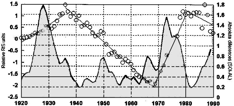
However, extratropical systems are not as well studied as ENSO variations, thus information on their relative importance for determining global variability is scarce in most cases. One exception is the Aleutian Low Pressure System, a dominant meteorological feature in the winter and spring North Pacific atmosphere that has strong links to North Pacific oceanography (Namias 1969). Figure 21 shows the smoothed Aleutian Low normalized sea level pressure (AL), together with the smoothed SOI series. Viewing their interdecadal variability, it seems evident both systems show parallel trends for most of the time, the exceptions being two periods during the late 1920s and early 1970s. These periods of unrelated behavior are more evident when looking at the absolute differences between both indices, in the bottom panel of Figure 21.
Figure 21. Upper panel: Transformed (standardize/I 1-year moving average smoothed) series of SOI and AL indices. Lower panel: Absolute differences between transformed SOI and AL series.
As mentioned at the introductory section, the origin of decadal-scale variability has been attributed to both the tropical and the extratropical systems by different authors, and to date no definitive conclusions have been reached. The controversy can be summarized as follows: whereas the identification of decadal signals in ENSO indices is considered by some (Graham 1994, Jacobs et al. 1994, Zhang et al. 1996) as strong evidence supporting the idea of a tropical forcing, some modeling results suggest that realistic simulations of extratropical variability of the North Pacific can be generated even without any input from the tropical Pacific system (Latif and Barnet 1994, 1996; White and Cayan 1996). If tropical forcing is to be considered the main source of extratropical variability, we would expect a parallel behavior of the series shown in Figure 21; these parallel trends do seem to occur generally but not all the time. Therefore, we believe the SOI-AL relationship is significant because it suggests the tropical forcing of the extratropics is not a constant mechanism.
Figure 22 shows the series of absolute differences between the SOI-AL indices together with the transformed sunspot numbers series. Results strongly suggest an inverse relationship between the two series, with the observed negative correlation coefficient (-0.5) being statistically significant. Therefore, large (small) SOI-AL absolute differences seem to occur during periods of low (high) solar activity. Assuming the degree of coupling of the tropical and extratropical systems could be reflected by a gross index such as the SOI-AL series, our results would suggest that those periods of relatively high solar activity tend to promote this coupling and therefore result in small SOI-AL differences. Somewhat independent tropical-extratropical variability (and therefore large SOI-AL differences) would tend to occur during periods of moderate to low solar activity. However, the effects of solar variability on the climate system of the earth are still a matter of controversy.
Figure 22. Upper panel: Absolute SOI-AL differences (lighter line) and detrended 11 year moving average anomalies of number of sun spots (area; data from the Sunspot Index Data Center-Royal Observatory of Belgium). Lower panel: Regression line and correlation coefficient between transformed Sunspots signal (x-axis) and absolute SOI-AL differences (y-axis).
Figure 23 shows the SOI-AL series as compared to the RIS regimes. These latter are identified by regression lines showing the general trends during selected periods. Periods when the SOI-AL differences are large tend to be of sardine (anchovy) population growth (decline), while anchovy (sardine) growth (decline) periods tend to occur when the SOI-AL differences are small. From the previously suggested relationships, it would follow that sardine growing periods (upward RIS trends) would tend to occur during years of diminished solar activity, when the tropical and the extratropical systems tend to behave independently. Anchovy growing periods (downward RIS trends) would take place during periods of increased solar activity and coupled tropical-extratropical interdecadal variability.
Periods of low (1941 to 1961) and high (1971 to 1977) differences of the SOI-AL series were used as reference periods for computing departures from the seasonal cycle of sea surface temperature (SST), sea level pressure gradient, and thermocline depth within selected systems (Figure 2). Figures 24 and 25 present the results of the analysis for the SST variability. Figures 26 and 27 those of pressure gradient, and Figures 28 and 29 those of thermocline depth.
SST results for most systems where large populations of sardines and anchovies grow suggest that periods of large SOI-AL differences (1971 to 1977) tend to be warmer than those periods when the tropical and the extratropical indices show parallel trends (1941 to 1961, when the SOI-AL differences are relatively small). California, Japan, Humboldt, and the Canary systems seem to behave this way. The only exception is the Benguela system where no difference between periods seems particularly evident. A similar tendency is also noticeable for the Eastern Tropical Pacific, whereas other systems such as Australia, Brazil, and Somali tend to behave in the opposite way.
Figure 24. Seasonal climatology (1: winter, 2: spring, 3: summer, 4: fall) of SST for the nine boxes shown on Figure 2. Base period: 1900 to 1990.
Figure 25. Seasonal departures (1: winter, 2: spring, 3: summer, 4: fall) of SST for the nine boxes shown in Figure 2. Referenced periods: 1941 to 1961 (solid circles) and 1971 to 1976 (open diamonds).
Figure 26. Seasonal climatology (1: winter, 2: spring, 3: summer, 4: fall) of SLP indices for the nine boxes shown in Figure 2. Base period: 1900 to 1990.
Figure 27. Seasonal departures (1: winter, 2: spring, 3: summer, 4: fall) of SLP indices for the nine boxes shown in Figure 2. Referenced periods: 1941 to 1961 (solid circles) and 1971 to 1976 (open diamonds).
Figure 28. Seasonal climatology (1: winter, 2: spring, 3: summer, 4: fall) of thermocline depth for the nine boxes shown on Figure 2. Base period: 1900 to 1990.
Figure 29. Seasonal departures (1: winter, 2: spring, 3: summer, 4: fall) of thermocline depth for the nine boxes shown in Figure 2. Referenced periods: 1941 to 1961 (solid circles) and 1971 to 1976 (open diamonds).
However, the described pattern is not evident from the thermocline depth analysis. Whereas this feature tended to be shallow in California and the Eastern Tropical Pacific during the 1971 to 1977 period, it tended to be deeper in Japan and Canary, and no clear tendencies are evident for the other systems where large fisheries of small pelagics occur (Humboldt and Benguela). At this point, it is not clear whether this lack of a coherent pattern is the result of the particular dynamics of each system or an artifact related to data scarcity. Similar ambiguous results were obtained for the pressure gradient analysis. Despite that differences for most systems seem to occur between the selected periods, no coherent pattern is observed. It is evident that proper evaluation of the interdecadal variability at the regional level will require more detailed approaches than the general analysis intended within this work.
![]()
![]()
![]()