10.1 Data Handling and Processing
10.2 Derivation of Estimates
10.3 Statistical Implications and Limitations
Echo-integrator surveys generate large amounts of data which must be manually reduced if in analog form, or by computer if it is digital. These data may be processed during the course of the survey if the research vessel has sufficient space and is suitably equipped. If this is not possible the data must be stored carefully for processing on shore later.
The quality of these data depends partly on care in their collection so it is particularly important that the following points are strictly monitored.
a. Ensuring that data entry on acoustic log sheets is consistent and correctb. Checking that instrument controls are properly monitored by all scientific personnel (observers) responsible for the acoustic watches
c. Correcting for 'drift' in the integrator, see 9.2.5 a phenomenon specific to the analog design of circuits, and to correct for factors such as: 'bottom pulse failure', see 9.2.1; 'layer selector spike', see 9.2.2; 'secondary echo interference', see 9.2.4 and 'blocking of integration due to a school generated bottom pulse' see 9.2.3
d. Eliminating false echo integrals attributed to various sources of noise, plankton layers and/or other scattering entities that may interfere in the measurements.
Whilst (a) and (b), can be considered self-explanatory and straightforward, (c) is rather complicated. A detailed description of the possible errors under (c) and some corrective measures for them are given in section 9.2. As for (d) this involves a comparison of echograms and integrams as explained in 10.1.1.
Chapter 10 deals only with post-survey, shore-based processing of analog data. Figure 90 shows the main elements in the system for processing analog integrator data. Satisfactory data processing and the derivation of absolute fish abundance estimates also depend to some extent upon the observer's subjective interpretation of the various displays as well as his ability to relate the measurements obtained to complementary biological samples. This involves a complex human decision making process, directly influencing the final abundance estimate as inferred from Figure 90. The quality of these decisions is necessarily dependent upon the observer's skill and experience in the interpretation of the acoustic data displays.
Figure 90. Outline of system for data handling and processing
The nature of survey data are such as to make it imperative that they first be studied and verified. Both echo-sounder records, integrams and log sheets are also subjected to careful scrutiny.
The purpose of this type of evaluation is twofold,
i) to carry out corrections for possible errors under (d) as defined above and,ii) to compare fish trace characteristics with the graphic integrator output (which represents a direct density index) in order to separate recorded biomass into discrete species and/or into plankton and fish.
In practice the most efficient way of comparing the two displays is to spread the echograms/integrams side-by-side (e.g. on a long table) so that 10-20 nautical miles of a transect can be viewed simultaneously. The advantage of such an over-view is that it often permits the detection of specific and important trends in data that might otherwise escape observance. Such trends can, for example, relate to a gradual appearance of a plankton layer which at some point will become mixed with the fish layer or schools of interest. In this case, careful examination of the long distance changes in trace characteristics, and correlation with the slope of the integrator output graph, often makes it possible to introduce reasonably accurate corrections. A similar approach also applies to other phenomena like secondary bottom-echo interference and even sea-surface noise which may have gradually built up to interfere significantly with the acoustic measurements.
The second purpose of the visual evaluation is to compare the acoustic displays with the related catch samples, e.g. in the form shown in Figure 91 (from Johannesson and Vilchez, 1979). Experience gained in many FAO projects demonstrates that such a comparison can significantly assist in the process of assigning echo-integrator values to a particular fish species. This can help to delineate their individual geographic distribution in areas where catch samples are scarce or simply not available.
A successful completion of the first two stages of data analysis described above, will result in a 'clean' set of integrator values (M), i.e. a clearer interpretation in terms of fish species and quantities. The third stage is to plot the M values. For an analog integrator the relationship between the M values and each survey sample represents a quantity defined by two coordinates relative to the water surface (latitude and longitude) and one scalar property, that is, the M-value, in millimetres, for example. A multi-channel integrator also offers a third coordinate, the depth.
A typical chart showing an actual track pattern from a large-scale survey together with the plotted M values is presented in Figure 92. With the survey data processed in this form, subsequent analysis normally proceeds along two lines, i.e. one aimed at data presentation and the other to derive absolute abundance estimates as shown schematically in Figure 90.
The purpose of data display and presentation is generally twofold; firstly to exhibit the survey results in a suitable form for the customer (e.g. fisheries managers). Secondly, to search for a better interpretation of data to realize their full potential which may significantly aid studies of trends and time-series, also correlation. With powerful mini-computers becoming commonplace, acoustic data display and presentation is rapidly developing in detail and sophistication.
For an illustration of this subject a summary of typical data presentations, partly reflecting the evolutionary changes over the past years is presented below.
A. Biomass distribution charts
i) Geographic Maps: Perhaps the most common way of mapping at present is shown in Figures 93 and 94. The first figure relates to a large volume pelagic stock along the coast of Peru, whilst the second one maps a relatively dispersed lake population. The difference in levels of the relative abundance categories should be noted but, otherwise the figures are self-explanatory.
Figure 93.
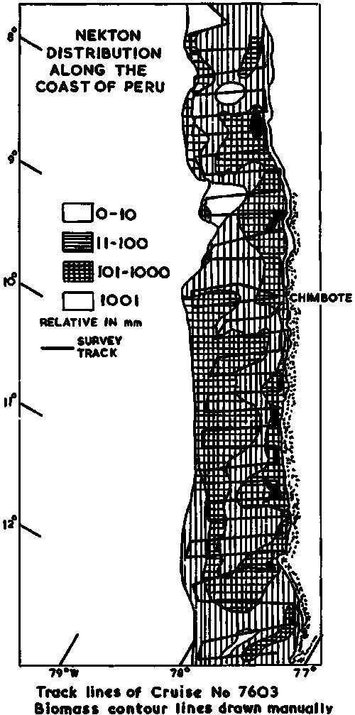
Figure 94. The geographic distribution of fish in Lake Titicaca estimated on the basis of 4 density categories
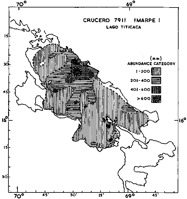
ii) Bar Graphs: These are also a fairly common form for data presentation.Figure 95 presents the same data as in Figure 94 but now in the form of a bar-graph. Such graphs, in a different fashion, can also be used to display biomass variations along a vessel's survey track-lines as illustrated in Figure 96 which is self-explanatory. A further construction of a bar-graph by a mini-computer facility is shown in Figure 97.
iii) Three-dimensional representation: This type of computer plotting is shown in Figure 98 below and refers to part of the same data presented in the form of a geographical distribution map in Figure 93,
Figure 98. All integrated echo intensities censored above a value of 1000
A somewhat different three-dimensional plot is shown in Figure 99 below.
B. Abundance profiles
i) Within-survey variability: An example of graphic analysis to study within-survey variations in echo-abundance by degree of latitude, as a function of the distance from the Peruvian coast, is shown in Figure 100 along-side.
Figure 100.
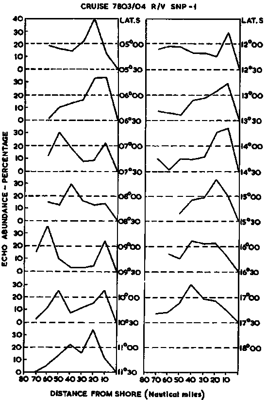
Figure 101. Distribution characteristics of Peruvian anchovy
ii) Survey-to-survey comparisons: This type of data presentation is particularly useful to study the characteristics of the littoral distribution of large volume pelagic stocks. An example from the Peruvian anchovy stock is shown in Figure 101. Data from eleven survey cruises are individually graphed to facilitate comparison with results from one survey to another, conducted over a period of four years. The principal area/density/weight magnitudes of the surveys are portrayed separately, using units of averages per degree latitude as the variate. In this form data lends itself to visual examination to judge whether any stationary pattern exists. If so it could serve as a basis for a better statistical survey design, e.g. to define some natural strata and/or to adopt probabilistic sampling allocations. A further display of these data is in Figure 102 where the principal survey variates are graphed to study seasonal changes in the area/density/biomass relationships.
C. Diurnal Variability
In ten years or more of integrator surveys it has been noted that significant differences can occur in the night/day ratio of integrated echo intensities returned from the same stock in the same area. Hence, it is commonplace in today's surveys to examine the extent to which such differences may influence an estimate and how a statistical compensation can be applied. In this case also a graphic analysis can aid the process. Clearly, numerous types of graph could be constructed in an attempt to elucidate the diurnal variability, but only three such examples are included in this manual. These are shown in Figures 103-4-5 which illustrate the night/day differences by hour, by day/night and by density stratum.
10.2.1 Scaling Factor 'C'
10.2.2 Simple Random Sample
10.2.3 Post-Sampling Stratification
The previous section dealt with analytical procedures leading to results in the form of distribution maps and graphs, whereas the present section deals with numerical analyses for the derivation of stock estimates. Referring to Figure 90, this takes us back to the plotted chart of M observations presented in Figure 92. In Chapter 6 of this manual, we saw that the equation for fish biomass (WB) of a given species within an area A, can be written in a simple form (Midttun and Nakken, 1977)
(88)
where C is the integrator scaling factor for the target species and  is the mean integrator value within the planimetrically integrated area A. The alternative way for numerical derivation of biomass estimate from a data base as plotted in Figure 92, is to employ the relationship
(89)
The first factor in the above product represents a rewriting of equation 59 from 6.4. This form for the estimation of biomass relies on a step-by-step calibration of the integrator system together with a knowledge of mean target strength for the relevant fish species. In the following, only equation 88 and its implications will be discussed.
The different methods for establishing the scaling factor C were detailed in Chapter 6 and the implications of the associated errors specifically treated in 9.4 of this manual. It is also important to be aware of biological processes that can play a significant role in the accuracy and the range of application of a given C value. To examine the problem more closely it is convenient to distinguish between four cases as follows:
a. C obtained from a technically successful live fish calibration experiment on a representative sample in terms of species and size distribution.b. C established for one particular species but applied to another species of similar size distribution (caution is needed).
c. C established for one narrow size-class, say, 19-20 cm but applied for the entire target stock with size distribution from 6-20 cm.
d. C obtained for one particular species of small size but also used for several larger species in the same survey area.
An evaluation of the above cases would first conclude that case (a) can be considered free of direct biological implications. As for (b), since the species are of similar size, a bias in C could arise as a result of differences in morphology particularly in relation to the swimbladder. Consequently, such differences should be investigated to assess the accuracy of using C for the second species.
In regard to (c) and (d) the broad application of C can be significantly influenced by length-dependent biases so that some correction will be required. Also, in case (d) morphological factors may introduce further bias if these are not taken into account.
The length-dependence of the scaling factor C is of great importance in acoustic stock assessment work and a better understanding of this relationship is necessary for control and correction of potential errors. A review of the theory, followed by a case study based on data from the Icelandic capelin research, illustrates the principles involved. First, we recall equation 56
r vD R = M/GeCi (s /4p)
which, for the present purposes, we can write in the form
r v = K (M/s)
where K represents a lumped constant. We are interested in the cross section per unit weight, i.e. (s /4p)/W where W is the weight of the fish. The weight/length and the cross-section/length relationship can be expressed as follows:
and
where l is the length of the fish species.
Substituting in the above equation gives:
(90)
Cross-section per unit weight can be misleading because P1 »
2.5 and P2 » 3. If  ,
r v is exclusively a function of M
but usually (P2 - P1) ¹
0 so the density estimator becomes length dependent. Clearly this can be corrected
if the functional relationship between l and the two variables (s,
W) is known. For the weight this is usually the case, while for the scattering
cross-section (s) this may require a special
investigation. It is better though to use TS per fish where the fish length
is in cm, then
TS = m log l + b
where m » 20 and b is a constant related to species and acoustic frequency. However, with increasing knowledge of the TS/length relationship in the form of published data, it is generally feasible to adjust the scaling factor C for variations in fish length. One approach, which has found application in investigations of the Barents Sea capelin stock (Nakken and Dommasnes, 1975) is to operate with a collective constant C' which mathematically is expressed as a function of individual scaling factors C1, C2, C3......Cn and the proportional length groups (year-classes) obtained from catch samples. To explain the principle involved in detail, let the individual densities of several year-classes be denoted by:
 when measured along a vessel's
survey track, or in a given survey area. We define the integrator reading M'
as the value produced collectively by the n year classes and the proportion
of each class: K1, K2, K3..... Kn
so that their total sum equals one, i.e. (K1 + K2 +.....
Kn) = 1. Given the above definitions, it can be shown by simple algebra
that
(91)
where the constant C' is given by the expression
C' = (K1/C1 + K2/C2 + K3/C3..... Kn/Cn)-1 (92)
An example of the practical application of this method is given below using data from joint Icelandic/Norwegian surveys of the Icelandic stock of capelin (Vilhjalmsson et al. 1982). From these data:
as illustrated graphically in Figure 106.
Figure 106. (a)
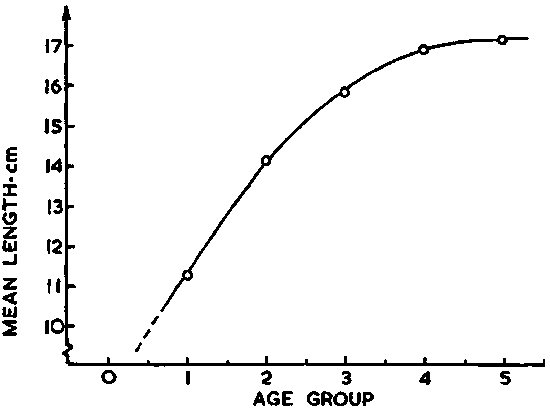
Figure 106. (b)
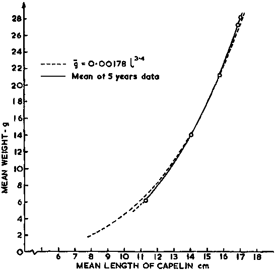
Secondly, the scaling factor Cf expressed in terms of numbers of fish per square-nautical mile referred to 1 mm integrator deflection is related to fish length as follows:
Cf = 8.1 x 10⁶ x l-1.91 (fish/mile2/mm)
Hence, the scaling factor Cf expressed in terms of biomass is readily calculated from
Using this expression and the graphic data in Figure 106a we can calculate the scaling factor C for the mean length of each year-class as follows:
|
age-group |
mean length (cm) |
scaling factor |
|
1 |
11.3 |
C1 = 0.534 |
|
2 |
14.1 |
C2 = 0.743 |
|
3 |
15.8 |
C3 = 0.880 |
|
4 |
16.9 |
C4 = 0.973 |
|
5 |
17.1 |
C5 = 0.990 |
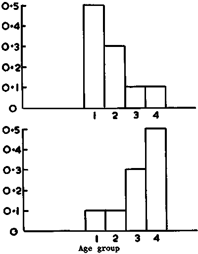
The theoretical variations in C with length is further illustrated by a self-explanatory set of graphs presented in Figure 107. Given that our main interest is to examine the overall theoretical variability in the collective constant C' (equation 92) we can adopt four hypothetical catch samples with distinct age-group compositions as shown in Figure 108. A set of K1, K2, K3 and K4 values is readily deduced for each of the four samples. Using the corresponding values of C1, C2, etc., and equation 92, the resulting values of C' can be calculated.
Figure 107.
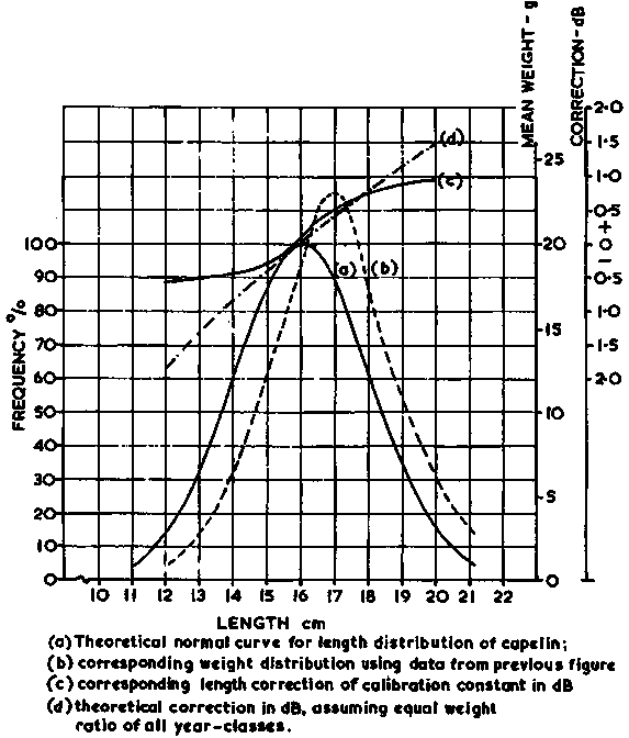
Repeating for the three remaining samples we get
The relatively modest level of variability in the above test values (C.V. = 11.7% about a mean of 0.759) suggests that, unless there are major changes in length frequencies from one sample to the other, the numerical value of C' remains relatively constant. But it also becomes evident that if the population being surveyed has for example a bimodal size distribution, appropriate corrections of C' would become essential.
The successful application of a length dependent scaling factor C' as defined above requires that (a) frequent catch samples be taken during a survey, (b) the samples be representative and thus free of bias due to gear selectivity. With these criteria fulfilled, the variations in C' (with species, length-group and their proportional weighting factors) can be calculated on the basis of equation 92.
Figure 108. (a). Proportional weight ratio of year classes of capelin
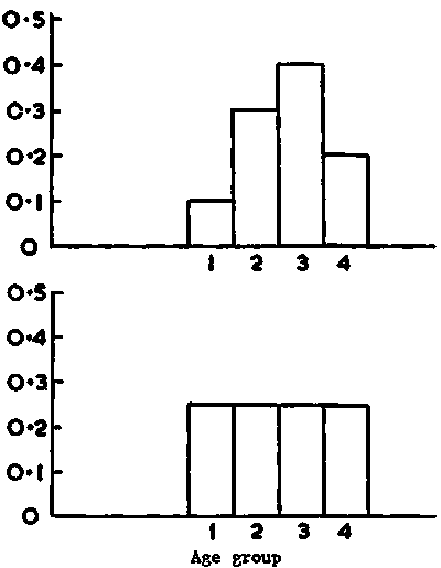
Figure 108. (b). Proportional weight ratio of year classes of capelin
We recall that the estimator for biomass (WB) in a given area (A) is commonly expressed in the form
This expression implies that if the scaling factor C, and the area A, can be
accurately determined, and also a representative mean value  can be derived, then an unbiased estimate of WB will result. Referring
to Figure 92 the problem is to estimate the parameter
  from the plotted set of data M1, M2, M3....Mn,
where each sample value is considered a statistically independent estimate of
the relative biomass. If these samples represent a truly random and representative
selection from the target population, an unbiased estimate of the population
mean would be given simply by
i.e., the random sample mean. However, this is rarely so with acoustic survey data due to the systematic nature of the sampling. Biological situations contain contagious distributions which are random, the fish are randomly distributed within groups and the groups are randomly distributed.
The set of data shown in Figure 92 demonstrates the possible level of bias involved by first treating the observations (Mi) as a simple random sample and then in 10.2.3 to re-calculate the estimated magnitudes on the basis of a stratified random sample for comparison. Two approaches can be adopted for the simple-random-sample estimate, often referred to as the geometric versus the algebraic method, depending on the way in which the population distribution area is determined. The two methods can be described as follows:
i) Algebraic Method
The basic principle is schematically illustrated in Figure 109. Each sample observation (Mi) is assigned to a corresponding rectangular area, here called "elementary statistical sampling rectangle" (ESSR).
Figure 109.
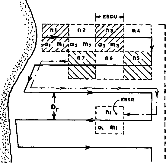
For a parallel survey grid with equidistant inter-transect spacing (DT) all ESSR's will have equal area sizes given by
ESSR = DT x (ESDU) mile2
where ESDU is the selected "elementary sampling distance unit" as described earlier. When the inter-transect spacing equals one ESDU, it follows that the ESSR becomes a square of size (ESDU)2. Given that zero observations (Mi = 0) are also counted then the total area A, is calculated as: A = a1 + a2 + a3 + .........aN, or
where N is the total number of ESSR's. Likewise, the mean of all observations is given by
and the total biomass
It should be noted that the area is determined as the algebraic sum of all ESSR's and hence the algebraic method.
ii) Geometric Method
The calculation of the mean is done in the same way except that only values of Mi ¹ 0 are counted, hence
where N is now the total number of actual biomass observations.
The total biomass is then given by
where the total area of distribution, A, is determined through geographic integration, e.g. by using a planimeter.
Applying the latter method to the plotted survey data of Figure 92 we obtain

Hence, the percentage bounds are ± 21.1% of the mean which can be compared with the stratified estimation procedure discussed in section 10.2.3.
The corresponding area size and scaling factor was
C = 0.78 tonnes/nautical mile2 per mm
A = 16,500 nautical mile2
So, in terms of biomass (WB)
Thus, giving lower and upper limits:
C.I. = (2,316,600 - 3,557,268) tonnes
An a priori stratification of sampling effort is difficult to achieve, (section 8.2 on the "Planning and Design of Surveys"). Consequently, a post-sampling stratification is commonly applied with the aim of increasing the precision of acoustic biomass estimates. Such a procedure is particularly expedient for survey data exhibiting heterogeneous distribution in terms of mean density and variance. Provided it is possible to divide the survey observations (and hence the surveyed fish population) into strata of greater homogeneity, the level of precision for interstratum estimates will be enhanced. Estimates of total biomass, with improved precision, are then obtained by combining estimates for all strata.
An attempt to post-stratify sample observations should begin with a study of their frequency distribution. Figure 110 shows a graphic illustration of the frequency characteristics of data used for calculation of the random sample mean in the previous chapter. Intuitively, the extreme positive skewness of the frequency distribution makes it unrealistic to adopt an arithmetic mean as a representative parameter. Also, a visual evaluation of the histogram does not suggest any natural division of these data. When this is the case and observations are wide ranging, it is customary to establish strata on the basis of logarithmic divisions as shown in the example below:
|
Stratum (h) |
M-values (mm) |
Abundance description |
|
1 |
1-10 |
very scattered |
|
2 |
11-100 |
scattered |
|
3 |
101-1000 |
dense |
|
4 |
1001-10000 |
very dense |
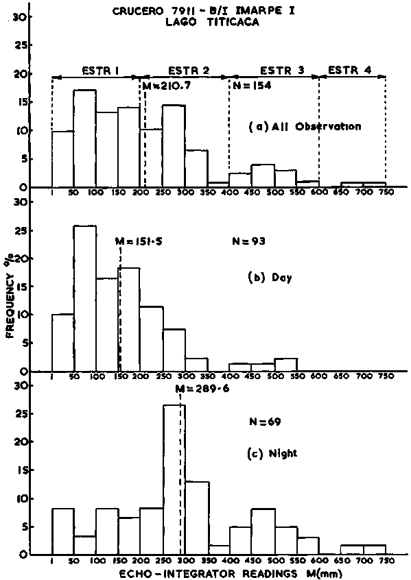
In other types of surveys, the frequency plots can give direct guidance to the selection of strata size and numbers as in Figure 111; the frequency distribution of data obtained during a survey of Lake Titicaca, Peru, (Johannesson, 1981). Figure (a) shows a set of four strata established on the basis of visual evaluation of the overall data histogram. The estimate resulting from these data demonstrated a relatively high level of precision (C.I. ± 4.5%, p = 0.95). Once the strata have been formed, the estimation procedure is as follows: First define the echo abundance (E) in the area, i.e.  , where A is defined by the density isolines. Because we are post-stratifying the M-observations for analytical purposes, it often happens that a given stratum, by our definition will result in more than one separate geographic area when the corresponding M isolines are constructed. For example in Figure 94 where the 3rd stratum (401-600 mm) has turned into six separate areas which we call sub-areas. Hence, the 3rd stratum comprises six sub-areas and the size of the stratum area is the sum of these. In practice, the area sizes are calculated by way of planimetric integration.
Figure 111. Frequency distribution of integrated echo intensities
The echo abundance  within
the jth sub-area, in the hth stratum is
(93)
where:
j = index for sub-area
n = number of M values within the jth sub-area
Aj = area size of the jth sub-area (mile2)
ith sample of M within the jth sub-area
The total echo abundance within stratum is found by summation
(94)
where m = number of sub-areas within stratum. Further, the total echo abundance in the area surveyed (Et) is found by the summation
(95)
where L is the total number of strata. Finally, the conversion into total biomass
 is obtained from the product
where C is the scaling factor as before.
Using the above method with data presented in Figure 110(a) we select the following strata:
|
Stratum 1: |
11-100 mm |
|
Stratum 2: |
101-1000 mm |
|
Stratum 3: |
1001-10000 mm |
Frequency histograms representing the individual strata are shown in Figure 110b,c,d and all 364 M-observations are tabulated, by stratum, in Table 10. A summary of the results of the relevant calculation is given as
Table 9.
|
Stratum (No.) |
No. of Samples |
Area mile2 |
Mean int. value |
Variance |
|
|
(nh) |
(Ah) |
|
|
|
1 |
174 |
9,200 |
47.5 |
3.7 |
|
2 |
178 |
7,000 |
274.8 |
195.0 |
|
3 |
12 |
300 |
2,157.1 |
174,315.0 |
|
Total: |
364 |
16,500 |
|
|
Total echo abundance 
Total biomass estimate 
Table 10.
Acoustic data corresponding to frequency histograms in Figure 110(b, c and d), used for calculation of stratified estimates
|
Stratum I |
n = 174 | ||||||||
|
Obs |
M |
Obs |
M |
Obs |
M |
Obs |
M |
Obs |
M |
|
1 |
26 |
37 |
48 |
73 |
64 |
109 |
54 |
145 |
62 |
|
2 |
34 |
38 |
48 |
74 |
27 |
110 |
80 |
146 |
41 |
|
3 |
18 |
39 |
10 |
75 |
19 |
111 |
54 |
147 |
19 |
|
4 |
19 |
40 |
11 |
76 |
27 |
112 |
89 |
148 |
24 |
|
5 |
55 |
41 |
12 |
77 |
21 |
113 |
70 |
149 |
51 |
|
6 |
56 |
42 |
65 |
78 |
11 |
114 |
71 |
150 |
55 |
|
7 |
18 |
43 |
60 |
79 |
24 |
115 |
54 |
151 |
13 |
|
8 |
10 |
44 |
18 |
80 |
82 |
116 |
66 |
152 |
66 |
|
9 |
50 |
45 |
35 |
81 |
96 |
117 |
70 |
153 |
22 |
|
10 |
75 |
46 |
19 |
82 |
85 |
118 |
82 |
154 |
13 |
|
11 |
70 |
47 |
41 |
83 |
60 |
119 |
75 |
155 |
80 |
|
12 |
93 |
48 |
37 |
84 |
41 |
120 |
28 |
156 |
51 |
|
13 |
45 |
49 |
83 |
85 |
49 |
121 |
86 |
157 |
12 |
|
14 |
25 |
50 |
90 |
86 |
11 |
122 |
20 |
158 |
80 |
|
15 |
63 |
51 |
91 |
87 |
24 |
123 |
27 |
159 |
82 |
|
16 |
41 |
52 |
69 |
88 |
16 |
124 |
55 |
160 |
50 |
|
17 |
19 |
53 |
61 |
89 |
87 |
125 |
42 |
161 |
68 |
|
18 |
3.8 |
54 |
82 |
90 |
72 |
126 |
59 |
162 |
34 |
|
19 |
84 |
55 |
40 |
91 |
59 |
127 |
10 |
163 |
40 |
|
20 |
52 |
56 |
24 |
92 |
25 |
128 |
30 |
164 |
13 |
|
21 |
55 |
57 |
64 |
93 |
23 |
129 |
13 |
165 |
17 |
|
22 |
17 |
58 |
90 |
94 |
30 |
130 |
71 |
166 |
20 |
|
23 |
83 |
59 |
15 |
95 |
35 |
131 |
21 |
167 |
10 |
|
24 |
67 |
60 |
47 |
96 |
54 |
132 |
93 |
168 |
20 |
|
25 |
70 |
61 |
29 |
97 |
30 |
133 |
57 |
169 |
12 |
|
26 |
24 |
62 |
52 |
98 |
21 |
134 |
87 |
170 |
27 |
|
27 |
75 |
63 |
54 |
99 |
88 |
135 |
45 |
171 |
19 |
|
28 |
21 |
64 |
42 |
100 |
59 |
136 |
64 |
172 |
19 |
|
29 |
12 |
65 |
44 |
101 |
28 |
137 |
40 |
173 |
38 |
|
30 |
30 |
66 |
27 |
102 |
75 |
138 |
37 |
174 |
74 |
|
31 |
16 |
67 |
62 |
103 |
76 |
139 |
24 |
|
|
|
32 |
54 |
68 |
68 |
104 |
28 |
140 |
16 |
|
|
|
33 |
82 |
69 |
75 |
105 |
34 |
141 |
87 |
|
|
|
34 |
69 |
70 |
91 |
106 |
77 |
142 |
77 |
|
|
|
35 |
83 |
71 |
75 |
107 |
35 |
143 |
17 |
|
|
|
36 |
79 |
72 |
83 |
108 |
56 |
144 |
31 |
|
|
|
Stratum II |
n = 178 | ||||||||
|
1 |
131 |
37 |
186 |
73 |
173 |
109 |
492 |
145 |
142 |
|
2 |
128 |
38 |
188 |
74 |
196 |
110 |
410 |
146 |
191 |
|
3 |
260 |
39 |
702 |
75 |
118 |
111 |
241 |
147 |
154 |
|
4 |
408 |
40 |
154 |
76 |
150 |
112 |
285 |
148 |
216 |
|
5 |
123 |
41 |
679 |
77 |
345 |
113 |
525 |
149 |
165 |
|
6 |
250 |
42 |
805 |
78 |
345 |
114 |
288 |
150 |
121 |
|
7 |
380 |
43 |
169 |
79 |
418 |
115 |
279 |
151 |
205 |
|
8 |
123 |
44 |
126 |
80 |
504 |
116 |
184 |
152 |
114 |
|
9 |
250 |
45 |
225 |
81 |
220 |
117 |
135 |
153 |
138 |
|
10 |
209 |
46 |
119 |
82 |
205 |
118 |
298 |
154 |
385 |
|
11 |
205 |
47 |
242 |
83 |
171 |
119 |
530 |
155 |
780 |
|
12 |
315 |
48 |
102 |
84 |
121 |
120 |
208 |
156 |
935 |
|
13 |
146 |
49 |
197 |
85 |
319 |
121 |
101 |
157 |
675 |
|
14 |
213 |
50 |
640 |
86 |
150 |
122 |
112 |
158 |
102 |
|
15 |
211 |
51 |
128 |
87 |
130 |
123 |
119 |
159 |
128 |
|
16 |
250 |
52 |
760 |
88 |
500 |
124 |
103 |
160 |
578 |
|
17 |
163 |
53 |
180 |
89 |
270 |
125 |
264 |
161 |
187 |
|
18 |
535 |
54 |
245 |
90 |
101 |
126 |
321 |
162 |
254 |
|
19 |
490 |
55 |
245 |
91 |
725 |
127 |
464 |
163 |
270 |
|
20 |
735 |
56 |
338 |
92 |
110 |
128 |
101 |
164 |
189 |
|
21 |
728 |
57 |
455 |
93 |
180 |
129 |
143 |
165 |
272 |
|
22 |
276 |
58 |
148 |
94 |
175 |
130 |
230 |
166 |
222 |
|
23 |
155 |
59 |
250 |
95 |
167 |
131 |
282 |
167 |
372 |
|
24 |
128 |
60 |
101 |
96 |
146 |
132 |
810 |
168 |
714 |
|
25 |
115 |
61 |
175 |
97 |
157 |
133 |
550 |
169 |
376 |
|
26 |
116 |
62 |
209 |
98 |
237 |
134 |
147 |
170 |
131 |
|
27 |
140 |
63 |
619 |
99 |
185 |
135 |
150 |
171 |
111 |
|
28 |
205 |
64 |
180 |
100 |
248 |
136 |
450 |
172 |
495 |
|
29 |
254 |
65 |
120 |
101 |
174 |
137 |
270 |
173 |
504 |
|
30 |
112 |
66 |
196 |
102 |
238 |
138 |
110 |
174 |
145 |
|
31 |
306 |
67 |
186 |
103 |
117 |
139 |
123 |
175 |
324 |
|
32 |
640 |
68 |
168 |
104 |
110 |
140 |
618 |
176 |
250 |
|
33 |
181 |
69 |
310 |
105 |
229 |
141 |
188 |
177 |
285 |
|
34 |
115 |
70 |
115 |
106 |
826 |
142 |
129 |
178 |
216 |
|
35 |
294 |
71 |
149 |
107 |
418 |
143 |
105 |
|
|
|
36 |
209 |
72 |
419 |
108 |
101 |
144 |
106 |
|
|
|
Stratum III |
n = 12 | ||||||||
|
1 |
1040 |
|
|
|
|
|
|
|
|
|
2 |
1375 |
|
|
|
|
|
|
|
|
|
3 |
1435 |
|
|
|
|
|
|
|
|
|
4 |
4655 |
|
|
|
|
|
|
|
|
|
5 |
1070 |
|
|
|
|
|
|
|
|
|
6 |
1150 |
|
|
|
|
|
|
|
|
|
7 |
1845 |
|
|
|
|
|
|
|
|
|
8 |
1920 |
|
|
|
|
|
|
|
|
|
9 |
3725 |
|
|
|
|
|
|
|
|
|
10 |
1340 |
|
|
|
|
|
|
|
|
|
11 |
1310 |
|
|
|
|
|
|
|
|
|
12 |
5020 |
|
|
|
|
|
|
|
|
Stratified variance estimate:
Confidence interval of the stratified estimate:
Thus, giving lower and upper limits:
C.I. = (2,101,502 - 2,590,412) tonnes
Hence, the percentage bounds are now reduced to ± 10.4%
Comparison of the results from the two different methods of analysis brings out two important factors,
(1) the stratification has produced a 10.7% gain in precision(2) the estimate of total stratified biomass is about 20% lower than the non-stratified result. This decrease in the point estimate attests to the fact that stratification also increases the accuracy of population estimates and ensures that subdivisions (strata) of the population are adequately represented.
It is instructive to compare the stratum graphs (Figure 110-b,c,d) with the
individual stratum variances as tabulated above. From the histogram for stratum
1, one would expect a low variance whilst for the heterogeneous character of
the frequency distribution in stratum 3, one would expect a high level of variance
which is confirmed by the coefficient of variance  for
the individual strata calculated as follows:
|
Stratum 1: |
C.V. = 14.6% |
|
Stratum 2: |
C.V. = 104.7% |
|
Stratum 3: |
C.V. = 12,050.0% |
These comparisons elucidate the importance of the formation of homogeneous strata for achieving satisfactory numerical biomass (population) estimates.
10.3.1 Transformation of Sample Observations
10.3.2 Confidence Limits for the Estimated Means
10.3.3 Allocation of Survey Samples
In 10.2 we applied two different approaches (stratified and non-stratified)
to derive point estimates for total biomass and then calculated the associated
statistical variance and confidence limits. Formulae from standard statistical
text-books, were used without qualification of their suitability for specific
methods of sampling and estimation. For example, it was assumed that the 'M'
as a variable would follow a normal distribution and hence symmetrical confidence
intervals about the estimated mean  would exist. Likewise statistical independence of the samples was assumed, thus
the effects of possible auto-correlation between the successive samples were
ignored. These and other factors of a statistical nature may significantly influence
the precision and accuracy of fish biomass estimates and, in particular, lead
to unreliable interval estimates (C.I.) if the methods of analysis are inefficient.
Much of the useful theory of sampling turns around the Normal Law, i.e. the normal distribution of Gaussian distribution defined by the equation
where m = mean and s = standard deviation.
Thus, for a valid statistical analysis of variance about an estimated mean ( , point estimate), the distributions must be of such character as to have means independent of the variance, i.e. to exhibit an approximately normal distribution. Distributions which depart seriously from the normal type (usually in fisheries acoustics by being excessively skewed in a positive direction), may require the technique of 'transformations' to be used to force the data into a better approximation to normality. Generally, this process can serve either or both of two main purposes to obtain
(a) a variable of increased practical relevance, e.g. for variance analysis(b) a variable with satisfactory approximation for further mathematical modelling of data, e.g. linear regression, or describe distribution patterns.
A full consideration of (a) and (b) require concepts too advanced for this manual so we deal with the first situation (a) with special reference to acoustic data. Only the typical positive skewness in acoustic data and the relevance of using transformations for their approximate normalization has been shown and two questions occur
(1) what is the criterion for transformations
(2) what type of transformation to insert for analytical purposes
It has been shown that regardless of the shape or form of a population distribution, the distributions of both the sum and the mean of random samples approaches that of a normal distribution as the sample size is increased. This statement is based on the important theorem known as the central-limit theorem. There is no absolute criterion as to how large the sample (n) must be for use in the normal approximation for computing the variance and confidence intervals. However, Cochran (1975), gives the following crude rule to determine the minimum sample size for populations exhibiting marked positive skewness
(96)
where G1 = Fisher's measure of skewness.
(97)
(E = expectation = product of sample probability times sample value).
This rule is designed so that a 95% confidence probability statement will be wrong for 6% or less of the time.
Type of transformation
When the sample is too small for the assumption of normality, a transformation is required. The choice of the correct transformation depends upon the original frequency distribution of the data, which is closely related to the spatial distribution of the fish stock from which data are collected. The spatial distribution pattern of fish concentrations are often characterised by their patchiness, or varying combinations of fish aggregations (clumpings) and layers of different densities. This is especially typical for larger pelagic fish stocks. Statistically, such distributions fall in the category of contagious distributions which can be expressed by several mathematical models, eg negative binomial, Polya-Aeppli, Neyman Type and Poisson distribution, as listed in order of decreased positive skewness (Elliott, 1971). Of these, the negative binomial distribution (with its two parameters m and the exponent k, and having variance greater than mean, (s 2 > m) has potential for use with acoustic data, since it can be derived from several mathematical and biological models and thus applied to a wide diversity of contagious distributions. The negative binomial distribution is probably the most suitable model for describing spatial distribution of fish stocks based on acoustic data because these data have a tendency to form a frequency distribution with extreme positive skewness. This, coupled with the fact that the logarithmic series is one of the most skewed of the negative binomial distributions (Elliott, 1971), often suggest a log-normal distribution. Consequently, the appropriate transformation is to form a new variate Mi = log xi, or Mi = log (xi + 1) in case the original variable Mi contains zero values.
More generally the appropriate transformations can be obtained from different distributions, eg Poisson, or the negative binomial distribution as shown in Table 11 below.
Table 11. Transformations obtained from the Poisson and the negative binomial distributions (given by Elliott, 1971).
|
Distribution | |||
|
Original distribution |
not known |
Transformation |
Special conditions |
|
Poisson |
|
replace x by |
No counts less than 10 |
|
Poisson |
|
replace x by |
Some counts less than 10 |
|
Negative binomial |
|
replace x by |
k* greater than 5 |
|
Negative binomial |
|
replace x by log (x + k/2) |
No zero counts |
|
|
|
replace x by log (x + 1) |
Some zero counts |
*k = exponent, interpreted as an index of clumping in the population
However, the general suitability is probably best expressed by Taylors Power Law Taylor (1961) which states that the variance s 2 of a population is proportional to a functional power of the arithmetic mean m. Thus
s 2 = am b
logs 2 = log a + b logm
Here, 'a' depends chiefly upon the size of the sampling units and 'b' is an index of dispersion which varies continuously from 0 for a regular distribution, to infinity for a highly contagious one. Once 'b' is determined, a common transformation can be applied to the original counts. The appropriate transformation is to replace each count by XP where p = 1 - b/2.
For a log normal distribution b = 2 and p = 0 so we should use a log transformation.
Thus if  , a = 1 and b = 2 p
= 1 - b/2 = 0
The advantages of b with respect to k are
i) the power law covers a wider range of distribution than the negative binomialii) the transformations derived from b are often easier to apply than those derived from the negative binomial (Elliott, 1971).
In this connection it can be briefly mentioned that if we make a log transformation such as Mi = log Xi, the so-called null hypothesis is
and the appropriate statistical test for the goodness of fit of a transformation is the c 2 (chi-square) test or alternatively the non-parametric Kolmogorev-Smirnov test. For a more detailed study of this subject, the interested reader is advised to consult relevant textbooks on statistics, e.g. Elliot, 1971; Kreyszig, 1970 and Massey, 1951. Also, Bazigos (1975) presents a c 2-test of acoustic survey data on Lake Tanganyika.
A practical understanding of the above comes by applying the log-transformation to data used in previous calculations of biomass and confidence intervals. First determine whether the sample size (n = 364) fulfills the criteria of eqn. 96. For this purpose we can use grouped data with class-intervals corresponding to the histogram shown in Figure 110(a). Hence, we take the mid-point of each class as a representative mean, moreover we let Mi = Xi. A summary of the relevant data tabulation is given in Table 12.
Using equation 97, the computations can proceed as follows:
Figure 112.


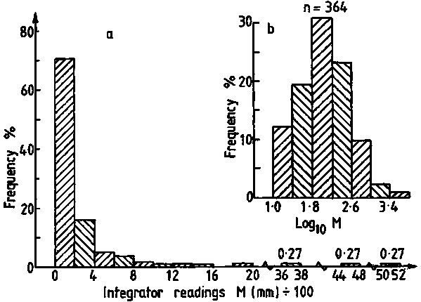
Table 12. Frequency distribution of 'M' using grouped data corresponding to the histogram in Figure 110
|
Class intervals D M |
(Mi = c i) c i |
Freq. fi |
fic i |
|
|
|
11 - 200 |
100 |
258 |
25,800 |
2,580,000 |
258,000,000 |
|
201 - 400 |
300 |
58 |
17,400 |
5,220,000 |
1,566,000,000 |
|
401 - 600 |
500 |
19 |
9,500 |
4,750,000 |
2,375,000,000 |
|
601 - 800 |
700 |
13 |
9,100 |
6,370,000 |
4,459,000,000 |
|
801 -1000 |
900 |
4 |
3,600 |
3,240,000 |
2,916,000,000 |
|
1001 - 1200 |
1,100 |
3 |
3,300 |
3,630,000 |
3,993,000,000 |
|
1201 - 1400 |
1,300 |
3 |
3,900 |
5,070,000 |
6,591,000,000 |
|
1401 - 1600 |
1,500 |
1 |
1,500 |
2,250,000 |
3,375,000,000 |
|
1601 - 1800 |
|
|
|
|
|
|
1801 - 2000 |
1,900 |
2 |
3,800 |
7,220,000 |
13,718,000,000 |
|
|
|
0 |
|
|
|
|
3601 - 3800 |
3,700 |
1 |
3,700 |
13,690,000 |
50,653,000,000 |
|
|
|
0 |
|
|
|
|
4601 - 4800 |
4,700 |
1 |
4,700 |
22,090,000 |
103,823,000,000 |
|
|
|
0 |
|
|
|
|
5001 - 5200 |
5,100 |
1 |
5,100 |
26,010,000 |
132,651,000,000 |
|
Totals: |
|
|
91,400 |
102,120,000 |
326,378,000,000 |

s 3 = (466.15)3 = 101,292,448
Hence, 
So finally
Considering sample size, we should have obtained at least 1253 observations
in order to apply the assumption of normal approximation. An additional factor
of interest from this calculation is the standard deviation of the grouped data
resulting in a numerical value s = 466.15 compared
with  for the non-grouped data
(see section 10.2.2). Some difference must be expected because of slightly changed
weighting effects related to the fact that we have taken the class midpoint
as a mean but not the within-class arithmetic mean. Given that our sample of
364 M-values is far too small to justify the assumption of normality, and that
the data are highly suggestive of a log-normal distribution, the next step will
be to apply the transformation
where  = midpoint value of
the classes forming the histogram shown in Figure 112(a). The distribution of
the transformed variate and some relevant preliminary calculations are presented
in Table 11. Also, a frequency histogram of the new variate (Zi)
is compared with the original data histogram in Figure 112(a-b). The normalizing
effect of the transformation is clearly demonstrated by the mode which has moved
from the extreme left to the centre of the apparent log-normal distribution.
For further analyses we continue as follows:
Table 13. Summary of Transformed Data
|
Interval class D c |
Midpoint class |
freq. fi |
|
Zifi |
|
|
11 - 200 |
100 |
258 |
2.00 |
516.00 |
1032.0 |
|
201 - 400 |
300 |
58 |
2.48 |
143.80 |
356.7 |
|
401 - 600 |
500 |
19 |
2.70 |
51.30 |
138.5 |
|
601 - 800 |
700 |
13 |
2.85 |
37.05 |
105.6 |
|
801 - 1000 |
900 |
4 |
2.95 |
11.80 |
34.8 |
|
1001 - 1200 |
1100 |
3 |
3.04 |
9.12 |
27.7 |
|
1201 - 1400 |
1300 |
3 |
3.11 |
9.33 |
29.0 |
|
1401 - 1600 |
1500 |
1 |
3.18 |
3.18 |
10.1 |
|
1601 - 1800 |
- |
0 |
- |
|
|
|
1801 - 2000 |
1900 |
2 |
3.28 |
6.56 |
21.5 |
|
|
- |
0 |
|
|
|
|
3601 - 3800 |
3700 |
1 |
3.57 |
3.57 |
12.7 |
|
|
- |
0 |
|
|
|
|
4601 - 4800 |
4700 |
1 |
3.67 |
3.67 |
13.2 |
|
|
- |
0 |
|
|
|
|
5001 - 5200 |
5100 |
1 |
3.71 |
3.71 |
13.7 |
|
Totals: |
|
364 |
36.54 |
799.1 |
1796.5 |
After having calculated the mean, variance and the standard deviation of the transformed data, the decoding would seem to involve straightforward antilogarithms giving, for example, a re-transformed mean
However, certain problems arise in transforming back in this way and we can note that the above derived mean (= geometric mean) is about 30% lower than the simple random mean M = 228.2 (see section 10.2.2). Embody (1952) recommends the use of the following formulae
where
= the mean of the transformed data
=the variance of the transformed data
= the adjusted geometric mean of the retransformed data
SA = the standard deviation of the retransformed data.
Adopting these we obtain
and
The results of applying such statistical corrections to the decoding process can be better evaluated through comparison with the results obtained from the simple-random-sample analyses as shown below:
|
Parameters |
Est. Mean |
Est. St. Deviation |
Coeff. Variation |
|
Data Treatment |
|
|
|
|
Simple random sample |
228.2 |
469.4 |
205.7 |
|
Log-normal distribution |
209.9 |
86.3 |
86.8 |
One will notice that the re-transformed mean gives a value of  ,
i.e. 8.15% lower than the simple random mean. The second effect of the log-normal
data treatment is a significant reduction in variability which in terms of coefficient
of variation is now reduced from 205.7% to 86.8%. Given these last figures,
the reader will also have noticed that we have already obtained four different
estimates of means from the same set of M-data; these are:
(1) Simple random sample mean:
(2) Effective stratified mean:
(3) Geometric mean:
(4) Adjusted geometric mean:
These estimates illustrate some of the statistical implications and limitations associated with estimation of representative means (central tendency of the data) from a set of acoustic data points. At the same time the importance of accurate statistical interpretations of the data and their analysis is emphasized.
In section 8.2.3 it was pointed out that when data from an integrator survey
are treated as statistical sample units, each observed integrator reading (Xi)
is conceived as an individual sample mean with its own underlying statistics ,
and the entire set of data as a sampling distribution of means. In such a case
the sample mean is given by
where n = number of integrator readings in the sample. The variance is then given by
and the standard error of the means
where s = standard deviation computed from the familiar formula
The standard error is a parameter of particular interest for the construction of confidence intervals about means since these are in fact expressed in terms of number of standard errors. This can be seen from the general expression for confidence limits, i.e.
where the values ± tc, called critical values or confidence coefficients, depend on the level of confidence (p) desired and the sample size (n). The numerical values for tc are found in Student's t-distribution (e.g. Pearson & Hartley 1966). Hence we may write
where tc corresponds to the desired probability level (commonly p = 0.95 or 95%) and (n-1) degrees of freedom. For relatively large sample size (n > 30), the coefficient tc can be replaced by another confidence coefficient zc, whose numerical values are found directly from the standard normal distribution for a given confidence level; thus for p = 0.95
and for 95% confidence level
More specifically we lay down our confidence limits as follows:
and
In sections 10.2.2 and 10.2.3 we calculated 95% confidence intervals for the
same set of data, first based on simple random sample then by post-sampling
stratification. Now we will derive the confidence limits yielded by the transformation
technique in the last section (10.3.1), from which we obtained the mean of log-transformed
data ![]() and the variance of log-transformed data
and the variance of log-transformed data .
Hence, we get
So,
Upper 95% limit = 2.4068
Lower 95% limit = 1.9932
Transforming back on the basis of direct antilogarithms gives
retransformed mean: 
retransformed Upper limit = antilog (2.4068) = 255.2
retransformed Lower limit = antilog (1.9932) = 98.4
Clearly, the resulting confidence limits are now asymmetric about the mean as can be shown by rewriting
The above limits can now be reconstructed, using adjusted antilogs based on the corrective formulae presented in section 10.3.1. From these formulae we obtain
Hence, the standard error of the retransformed data is now
and 95% confidence interval
C.I. = 209.0 ± 1.96 x 9.555 = 209.0 ± 18.7
with Upper limited = 228.6 and Lower limit = 191.2.
Earlier we obtained four different estimates of means (10.3.1), and have now calculated the associated confidence intervals using four different statistical approaches. Comparison of the results is facilitated by line graphs shown in Figure 113. Visual evaluation of these graphs indicates methods (b) and (c) as the most efficient estimators for the data mean, whose two estimates differ about 13%. As for methods (a) and (d), they differ considerably among themselves both with respect to the mean and confidence intervals (the latter, d, being asymmetric) and also vary significantly to the other two methods.
Figure 113.
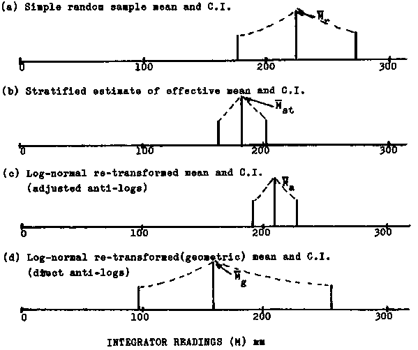
Line graphs for comparison of estimated means and 95% confidence intervals obtained from different data treatment
Consequently, it can be concluded that for highly skewed acoustic data, the stratified or the log-transformation procedure is likely to yield the best estimates. Which one of the two methods is better, will, on one hand, depend on how uniform strata can be formed for the stratified estimation procedure, and on the other hand, on how closely the log-transformed data will fit the theoretical normal distribution in the log-normal estimation approach. To determine the exact suitability in this respect may require some detailed statistical tests that are beyond the scope of this manual.
i) Estimates from Non-Skewed Data
So far the statistical calculation and estimates have turned around data characterized by marked positive skewness. The associated statistical problems have been demonstrated by a case study using real data from a survey of the Peruvian anchovy. We will now analyse another set of real acoustic data which is non-skewed and, intuitively, resembles a normal distribution as shown by the histogram in Figure 114. These data relate to an estimation of nekton biomass in the Strait of Bali, Indonesia, from an acoustic survey by R.V. TENGGIRI from 28 February-1 March, 1982. Figure 72 shows a map of the area covered and the survey transect pattern. The integrator readings in millimetres for each 2-mile section of the cruise track (ESDU) are given in Table 14. First, we analyse the tabulated data of Table 14 in a stratified random design using the algebraic method for determination of stratum areas. Thus, we proceed as follows:
Figure 114.
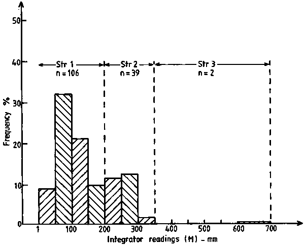
Table 14. Acoustic data observations grouped into three stratum corresponding to the frequency histogram shown in Figure 114
|
Stratum 1 (1-200 mm) |
n = 106 | ||||||||
|
Obs |
M |
Obs |
M |
Obs |
M |
Obs |
M |
Obs |
M |
|
1 |
95 |
23 |
25 |
45 |
200 |
67 |
89 |
89 |
106 |
|
2 |
83 |
24 |
8 |
46 |
116 |
68 |
73 |
90 |
122 |
|
3 |
34 |
25 |
20 |
47 |
80 |
69 |
70 |
91 |
150 |
|
4 |
73 |
26 |
71 |
48 |
110 |
70 |
108 |
92 |
182 |
|
5 |
45 |
27 |
138 |
49 |
124 |
71 |
157 |
93 |
145 |
|
6 |
63 |
28 |
112 |
50 |
65 |
72 |
78 |
94 |
80 |
|
7 |
188 |
29 |
115 |
51 |
102 |
73 |
119 |
95 |
109 |
|
8 |
93 |
30 |
73 |
52 |
65 |
74 |
112 |
96 |
104 |
|
9 |
113 |
31 |
23 |
53 |
25 |
75 |
61 |
97 |
79 |
|
10 |
109 |
32 |
55 |
54 |
164 |
76 |
60 |
98 |
57 |
|
11 |
83 |
33 |
145 |
55 |
84 |
77 |
82 |
99 |
38 |
|
12 |
82 |
34 |
179 |
56 |
63 |
78 |
72 |
100 |
53 |
|
13 |
112 |
35 |
20 |
57 |
73 |
79 |
100 |
101 |
52 |
|
14 |
105 |
36 |
68 |
58 |
168 |
80 |
107 |
102 |
62 |
|
15 |
78 |
37 |
99 |
59 |
200 |
81 |
135 |
103 |
82 |
|
16 |
69 |
38 |
186 |
60 |
101 |
82 |
154 |
104 |
106 |
|
17 |
67 |
39 |
59 |
61 |
92 |
83 |
90 |
105 |
99 |
|
18 |
62 |
40 |
152 |
62 |
52 |
84 |
74 |
106 |
65 |
|
19 |
76 |
41 |
133 |
63 |
114 |
85 |
54 |
|
|
|
20 |
100 |
42 |
140 |
64 |
147 |
86 |
36 |
|
|
|
21 |
42 |
43 |
165 |
65 |
149 |
87 |
46 |
|
|
|
22 |
68 |
44 |
197 |
66 |
129 |
88 |
71 |
|
|
|
Stratum 2 (201-350 mm) |
n = 39 | ||||||||
|
1 |
211 |
17 |
316 |
33 |
208 |
|
|
|
|
|
2 |
223 |
18 |
296 |
34 |
310 |
|
|
|
|
|
3 |
246 |
19 |
230 |
35 |
205 |
|
|
|
|
|
4 |
300 |
20 |
270 |
36 |
246 |
|
|
|
|
|
5 |
243 |
21 |
284 |
37 |
290 |
|
|
|
|
|
6 |
285 |
22 |
223 |
38 |
280 |
|
|
|
|
|
7 |
248 |
23 |
291 |
39 |
259 |
|
|
|
|
|
8 |
201 |
24 |
261 |
|
|
|
|
|
|
|
9 |
234 |
25 |
258 |
|
|
|
|
|
|
|
10 |
258 |
26 |
202 |
|
|
|
|
|
|
|
11 |
243 |
27 |
220 |
|
|
|
|
|
|
|
12 |
233 |
28 |
254 |
|
|
|
|
|
|
|
13 |
210 |
29 |
282 |
|
|
|
|
|
|
|
14 |
263 |
30 |
322 |
|
|
|
|
|
|
|
15 |
263 |
31 |
280 |
|
|
|
|
|
|
|
16 |
265 |
32 |
267 |
|
|
|
|
|
|
|
Stratum 3 (351-700 mm) |
n = 2 | ||||||||
|
1 |
670 |
|
|
|
|
|
|
|
|
|
2 |
635 |
|
|
|
|
|
|
|
|
Table 15. Estimation of biomass by cluster sampling
Stratum 1 (0-200 mm)
n1 = 106, A1 = (ESDU)2 x n1 = 4 x 106 = 424 mile2
Let Mi = xi, then we have: 

t.95 = 1.98 (from Student's t-tables)

Stratum 2 (201-350 mm)
n2 = 39, A2 = (ESDU)2 · n2 = 4 x 39 = 156 mile2


Stratum 3 (351-700 mm)
n3 = 2, A3 = (ESDU)2· n3 = 4 x 2 = 8 mile2


Combining the above results to find the stratified variance (Vst) we obtain

and the standard error: 
Effective stratified mean:

At this point it will be noted that the relevant confidence limits should be established in terms of echo-abundance (E = product of integrator value times area) because the stratified standard error now represents an area-weighted quantity. Since, however, the biomass weight is given by the product of the echo-abundance and scaling factor (WB = EC), the confidence intervals can also be established for the mean biomass estimate. The pertinent scaling factor was: C = 0.54 tonnes/mile2 per mm integrator deflection. Hence mean biomass estimate (i.e. point estimate)


* for df = (n1 + 1) + (n2 + 1) + (n3 + 1) = 144
giving Upper 95% C.L. = 48,279 and Lower 95% C.L. = 44,037
Resulting in percentage bounds of ± 4.6%
Our interest now is to re-analyse the same data in a simple random design for comparison with the above result.
ii) Simple random sample
With a scientific pocket calculator we obtain:
n = 147, A = 588 n.mile2 

and t.95 = 1.98 as before.

now giving Upper 95% C.L. = 51,470 and Lower 95% C.L. = 40,905 corresponding to percentage bounds of ± 11.4%.
Comparison of the stratified/non-stratified results, in relation to virtually non-skewed data, brings out the following points
(a) Both methods give almost exactly the same estimates for the data mean, thus the simple random estimator, in this case, can be considered unbiased.(b) The stratified estimator is more efficient since it gives considerably narrower confidence intervals (i.e. 4.6% compared with 11.4%) and hence, more precise estimates.
It will be noted that in the foregoing procedure and calculation of confidence intervals, only one variable has been considered, namely the integrator observation (Mi), alternatively denoted by x- for convenience. Recalling that 'M' is proportional to the product of fish density times back-scattering coefficient, i.e.
M µ r v x (s /4p )
it is clear that M contains components of variability related firstly to natural variations in fish density (behaviour) and, secondly, to variations in the reflectivity property of the fish which in turn depends on the fish size and spatial orientation pattern. In addition, it includes a certain component of variability associated with the measurement system itself. Consequently, the size of the confidence intervals are governed largely by uncontrolled variations directly related to the structure and dynamics of the natural population, but not so much attributed to the variability in the acoustic measurement method itself. To separate the latter component from the intrinsic variability in the population is obviously a difficult task. Theoretically it might be approached on the basis of experimental, replicate survey designs and assumptions of constant population size in a given area. Such an approach would require rare experimental conditions coupled with detailed analysis of variance of the results.
A different practical approach to the construction of in-situ confidence intervals was devised by Lozow (1973), where intervals at a given confidence level can be constructed as a function of the relative level of variability between r v and (s /4p ). The interested reader is advised to study Lozow's paper. Further discussion of the subject is beyond the scope of this manual.
iii) Confidence intervals vs. serial correlation
In the previous calculations, the assumption was made that the individual observations, M, represented statistically independent samples, implying that although the samples are normally obtained in a serial manner, they are expected to be free of serial correlation effects. However, several workers have shown that this assumption may not be valid. Bazigos (1976) estimated auto-correlation coefficients for different density strata of acoustic data obtained during an integrator survey of Lake Tanganyika in November 1973 pointing out that this would have inflationary effects upon the variance but did not suggest a correction. Nickerson and Dowd (1977) describing estimates of fish density realized that successive acoustic observations could be significantly correlated and thus result in an underestimate of the actual variance. To correct for this they used a model given by Hogg and Craig (1968).
where
variance estimate of the serial observations
, and
Pj = autocorrelation coefficient between a pair of observations j apart, 1 £ j £ n - 2
Shotton and Dowd (1975) examined the problem of variance estimation for acoustic data and suggested the use of a cluster sampling estimate of Hanse et al. (1953). Also, Williamson (1982) presented results from a computer simulation study designed to examine the effect of auto-correlation on the variance of the random sample estimate of m d and to evaluate the use of cluster sampling approach for estimating m d.
Further theoretical background will not be discussed in this manual, but in order to illustrate the importance of the serial correlation effects, we will now re-analyse the previous data (Table 14); using formulae from Williamson (1982).
iv) Analyses of data in a cluster design
The previous analysis assumed no serial correlation or this source of variance
was omitted. Estimated variance and the associated bounds on the point estimate
are therefore underestimates depending upon the extent of serial correlation.
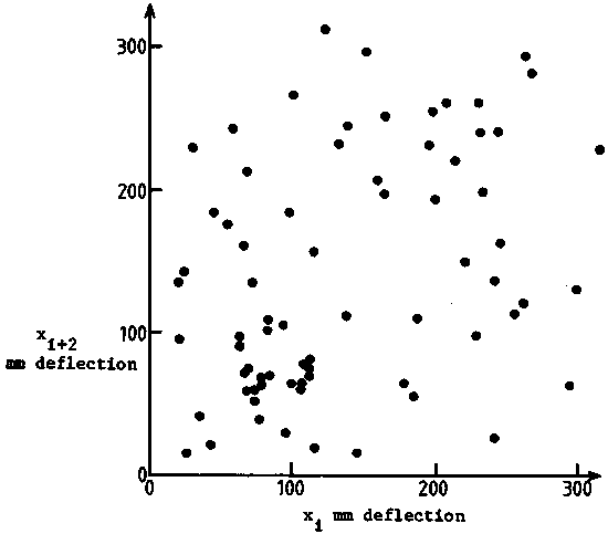
This was explored by two scatter diagrams of the observations viz. xi
versus xi+1 (Figure 115), xi versus xi+2 (Figure
116). While there is a high degree of correlation between one observation and
the next adjacent one x1+1, this correlation disappears between xi
and xi+1. In other words the auto-correlation function r(k) = 0 for
log k = 2. This fact must therefore be incorporated in the variance estimate
for the mean density  in the
surveyed area. An approximate expression from Williamson (1982) is:
Here
t = total number of transects
ni = number of observations within a transect i
N = total number of observations or
Di = sum of ni observations in transect i
Figure 115.
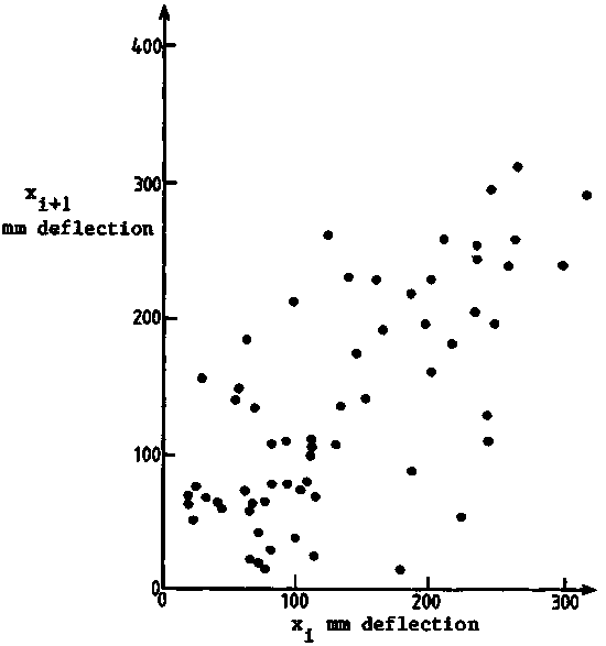
Figure 116.
These data are summarized in Table 15; 25 transects (clusters) are listed derived by adding the short connecting transect to the preceding long one perpendicular to the coast line.
The given variance estimate is an approximation but a rather good one when
the coefficient of variation (CV) of  is < 0.2
By using the data in Table 15 the calculated value became CV =.06 or well within the given limit.
By substitution of the values in Table 15 we obtain the necessary auxiliary quantities for substitution in the formulae for variance


= (1/1472) (25/24) {22,222,511 + 145.322.939-(2.145.31)(129,553)} = (1/21609) (1.0417) (42,049,492 - 37,650,693) = 212.05
The bounds on the point estimate, which is very close to the previously derived estimate (145.37) are in this case substantially increased.
Calculation of total biomass in tonnes proceeds in the same manner as before by using the scaling factor C = 0.54 tonnes/mile2/mm, and a total area estimate of A = 588 mile2. Thus, total biomass
And the corresponding bounds (B)
giving Upper 95% C.L. = 55.293 (48,279*) and Lower 95% C.L. = 36,985 (44,037*)
resulting in percentage bounds of ± 19.8%.
* from the stratified estimate
The important point brought out by these two principally different ways of computing the variance, is the substantial impact serial correlation has on the magnitude of the variance around the mean density. In fact it has more than trebled. This consists of both intra- and inter-transect serial correlation. The reality of the latter one is in this case explored by computing the correlation coefficient between Di and Di+k, where k = 1, 2, 3,..... etc., is the lag in number of observations between paired observations, e.g. Di and Di+3 when k = 3.
Thus, the auto-correlation coefficient rk measures the correlation between integrator readings k observations apart. The closer rk is to 1, the higher the degree of serial correlation in the sample. To the contrary, values of rk close to zero indicate little or no serial correlation in the sample.
The correlation coefficient for the intertransect (or inter-cluster) correlation, up to the 5th order was estimated from the approximate formula
The basic data for this formula are summarized in Table 16. By calculator
Using this result and the tabulated data we obtain
rk=1 = (1,778,427 x 25)/24 x 24 x 170,090 = 0.456
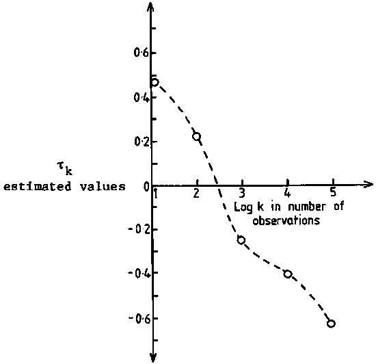
Repeating the calculation we can summarize the following results
rk=1 = +0.456
rk=2 = +0.218
rk=3 = +0.249
rk=4 = -0.415
rk=5 = -0.631
these are presented graphically in a correlogram (Figure 117).
Figure 117.
The fact that two closely spaced transects (= 1 ESDU in this case) show a positive correlation is expected intuitively since the serially returned observations (cluster returns) come from a fish population where natural forces are likely to induce a slow change, or even a trend, as we proceed from one transect to the next one, or from one ESDU to the following one. As a result, auto-correlation effects in acoustic survey samples may dictate the need to introduce a correction in the variance expression and this may significantly increase the estimated confidence intervals. As for the specific type of correction to be used, it is a subject under study by some writers and therefore difficult, at present, to define or recommend any optimum approach to the problem. However, it is noteworthy that Shotton and Dowd (1975) concluded that of the three methods they examined, only the cluster estimate of Hansen, Hurowitz and Madow (1953) appeared conceptually sound with respect to assumptions of the data.
If there is some knowledge of the expected nature of the overall variance, for example when planning a second survey in a given area, and if little change is expected in the nature of the sampling results, then the variance can be decreased by improving the allocation of sampling effort. Transects of greater length are preferred when the intra-transect correlation is high. When most of the variation occurs between transects, then more transects of shorter length would decrease the variance. If transects make parallel and complete crossings of the stratum then to this extent the transect lengths will be predetermined.
The acoustic data used for the two preceding case studies are related to systematic surveys with equidistant transect spacing. In such cases, the allocation will be proportional to the area sizes in each stratum. This section is intended to introduce the concept of 'optimum sampling allocation' and as a further development of the above case studies, to make comparisons between the proportional and optimum allocation of sampling efforts in stratified sampling.
The optimum allocation of survey effort refers to a sampling method that gives a minimum variance under the restriction (cost not considered) that the total sample size is n and that we have h strata. In this case, the number of samples per stratum, nh, is given by
nh = (n Ah Sh)/S h Ah Sh
Ah = size of the stratum area
Sh = standard deviation of the stratum sample.
Applying the above formula, the calculation can proceed as follows.
1) For the Skewed Data
From Table 9 we can readily compute the standard deviation
|
Stratum 1 |
: |
|
Stratum 2 |
: S2 = (V(M2))1/2 = (195.0)1/2 = 13.96 |
|
Stratum 3 |
: S3 = (V(M3))1/2 = (174,315.0)1/2 = 417.5 |
Further, S Ah Sh = A1S1 + A2S2 + A3S3 = 9200·1.92 + 7000·13.96 + 300·417.5 = 17,664 + 97,720 + 125,250 = 240,634.
Having obtained the relevant numerical values for substitution in the formulae for optimum sample size by stratum, we get
n1 = 364 x 17664/240634 = 26.72 @ 27
n2 = 364 x 97720/240634 = 147.82 @ 148
n3 = 364 x 125250/240634 = 189.46 @ 189.
The actual sampling allocation is compared with the estimated optimum allocation
Table 17
|
Stratum (No.) |
Sample allocation |
Difference (ratio) |
|||
|
Actual |
Optimum |
||||
|
n |
% |
n |
% |
||
|
1 |
174 |
47.8 |
27 |
7.4 |
6.5 times over-sampling |
|
2 |
178 |
48.9 |
148 |
40.7 |
1.2 times over-sampling |
|
3 |
12 |
3.3 |
189 |
51.9 |
15.7 times under-sampling |
|
Totals: |
364 |
100 |
364 |
100 |
|
The result shows that for the given criteria, only stratum 2 was adequately sampled, while the sampling allocation in the low density stratum (1) appears exorbitant and, to the contrary, the sampling effort in the high density stratum (3) is totally insufficient. Consequently, the variance could be reduced by a proper allocation of sampling within strata,
ii) For the Non-Skewed Data
Following the same procedure as above, we obtain the following result:
|
Stratum 1 |
: n1 = 106; A1 = 424; S1 = 4.24 |
|
Stratum 2 |
: n2 = 39; A2 = 156; S2 = 5.30 |
|
Stratum 3 |
: n3 = 2; A3 = 8; S3 = 17.50 |
Hence,
S Ah Sh = 424 x 4.24 + 156 x 5.30 + 8 x 17.50 @ 1798 + 827 + 140 @ 2765
So, the optimum sampling allocation is
n1 = 147 x 1798/2765 = 95.59 @ 96
n2 = 147 x 827/2765 = 43.97 @ 44
n3 = 147 x 140/2765 = 7.44 @ 7.
The comparison with the actual sampling is shown in Table 18.
Table 18.
|
Stratum (No.) |
Sample allocation |
Difference (ratio) |
|||
|
Actual |
Optimum |
||||
|
n |
% |
n |
% |
||
|
1 |
106 |
72.1 |
96 |
65.3 |
1.1 times over-sampling |
|
2 |
39 |
26.5 |
44 |
29.9 |
1.13 times over-sampling |
|
3 |
2 |
1.4 |
7 |
4.8 |
3.5 times under-sampling |
|
Totals: |
147 |
100 |
147 |
100 |
|
The result shows that for the kind of data in question, the actual allocation of the survey effort does not deviate very much from an optimum allocation, although stratum 3 appears insufficiently sampled. Hence, in this case, a change in the sampling effort is not likely to produce much reduction in the variance.