![]()
![]()
Age structure changes
Since we know already that an unexploited (by man) system will tend to comprise many older, high fecundity individuals with low-specific consumption requirements, it would appear that each species would tend to respond through long term selection to system perturbations such as changes in primary production rates, changing temperatures or even predation due to sporadically appearing nomadic predators, by promoting larger-older individual's abundance, increasing age classes, and generally shortening smaller, immobile stages as much as possible, i.e. maximizing growth rate and efficiency. Fisheries operate in opposition to this set of characteristics.
Whereas many pelagic fish species have managed to accomplish only the latter few things, many cannot reach large size and thereby decrease their predator field. Clupeids, engraulids and numerous bathypelagic species are in this group. However, some other species have evolved not only rapid growth, older-larger age classes, but also formidable sizes, i.e. the large sharks, the genera Seriola, Scomberomorus, Thunnus, Coryphaena, the istiophoridae and Xiphius gladius. These species are usually apex predators of omnivorous habit, high activity and mobility, and can be extremely ecologically inefficient (Sharp, 1983) in contrast with demersal or sedentary predators.
The opposite extreme is the situation for substrate specific populations, i.e., tropical reef fishes or tidal zone inhabitants where the populations are smaller in absolute numbers, life times are fairly short and even the size of potential predators is limited by the environment, i.e. refugia. Here the physiological and morphological adaptations for surviving the rigours of the environment are prerequisites. Variable growth or limited size, territorial behaviour, brooding or rearing of younger stages in those species with low fecundity, etc. are all demanded by “the Environment” if a species is to thrive. Yet the absolute adult population sizes are set by the number of appropriate home “sites”, or substrate occupied, because any other than those individuals “on site” and actively maintaining their tenancy will be washed away, preyed upon or otherwise kept from occupying permanently “a site”. What is interesting in this case is that exploitation of such species will open sites and tend to decrease natural mortality in the population at large, up to the point where fishing mortality is greater than the limiting “site” recruitment rate which will depend both on females “on site” as well as their abilities to produce sufficient young to fill any available sites. A reef fish assemblage may actually vary primarily in response to the very sporadic reductions of individuals in localized contexts which can also be subsequently recolonized by other, locally abundant species. This would make modelling reef fish communities very much more “fragile” than modelling either pelagic or demersal communities, due to the fact that as available substrate varies, reproduction rate varies as a function of “on site” individuals; natural mortality rate would tend to fluctuate as a function of fishery intensity and local predation intensity; and overall mortality would depend upon “open site” recolonization related to the number of species and recruiting individuals competing for the “sites”. This involves extremely complex feedback loops. It might well be more useful to assume that reef fishes of various habitats have tended to achieve similar growth and recruitment potential, and that knowledge of size-age structures and substrate area might actually give the best estimates of turnover rates, hence fishery potential in these cases.
BUILDING THE “UNDERSTANDING MODEL”
A numerical model is nothing else then a representation of an “understanding model” in the sense that it simulates and integrates our knowledge on the modelled processes. It will take into account the available facts and put in equation the hypotheses put forward in order to explain these facts. It will therefore be just as good or bad as our knowledge was. There is very likely a marine population to fit most conceivable models. We do not believe, however, that there is any single model to fit all fisheries, or that there is an available model for all fisheries.
The common denominators of neritic resources are difficult to identify, although some certainly exist in smaller time-space references. Our problem is that starting with any single resource upon which a fishery develops, how much and what kind of information is necessary to adequately and effectively “manage” both the distribution of fishing effort, and monitor the resource such that the effort appropriately tracks any changes in the resources' distribution, potential, or position in its milieu, the ecosystem?
This is not a simple question and there is no simple answer. The elements need to be examined in perspective, leaving only specific examples of individual species aside so as not to clutter the discussion with anecdotal material.
There is a fairly extensive historical log of the efforts of scientists (and philosophers) to unravel the marvels of the sea, e.g., Pliny and Aristotle's writings; the studies of Linneaus; and records of the age of exploration of the seas, culminating in Darwin's treatise on speciation. Astute marine biologists flowered at the turn of the twentieth century. Early insights of the Norwegians were documented by Hjort in his treatise of 1913–1914, and Graham's (1935) development of fishery statistics and continuing efforts to understand environmental effects of feeding, growth, maturation and early life history of fish are remarkable. It seems that few of us today have progressed beyond their insights. Of course, there have been remarkable re-developments of basic concepts, and subtle mathematical expressions devised to express them, but the problem of obtaining better insights into what causes the variations and how to cope with them has not been resolved, although we may be getting closer in solving some of the intermediate questions.
Early pioneers in fishery-oceanography like Kishinouye (1923) and Uda (1927, 1952) had already formulated relations between, for example, species morphology, physiological capabilities and oceanic variations, hence zoogeographic and fishery related behaviour. The importance of system variables, currents, temperatures, oxygen, food abundance, etc., although certainly recognized, have too often been taken in gross forms, i.e., average surface temperatures for a series of months, and these values have been “regressed” or “correlated” with fishery yields or recruitment. Short series containing correlated trends have been identified for numerous data pairs. Skud (1982; this volume) has also pointed out that they actually reverse under certain conditions, usually involving a change in dominance of one species with another, and the second species often takes on the response pattern characteristics of the first species upon which the correlations were based. This speaks clearly for opportunism in the face of a system-wide change of state.
Meanwhile, it is also important to recognize early on that fish are very much part of a larger system, loosely termed an ecosystem, which they, in turn, support various components of, and from which they extract their needs. The ecosystem is constituted of intrinsic (internal) components, and extrinsic ones. Time and distance scales are very significant in interpreting changes in the fishery catches, particularly as they might reflect effects of factors extrinsic to specific fishery geographies. Fisheries do not reflect only local events, but also climate-ocean and solar system driven changes, which induce biological ones. It is important to realize that within even these eco- system constraints the basis of all present modelling of populations is the “unit stock” assumption for each resource under study. Eventually, the questions arising from observed variations must be addressed with regard to any potential non-homogeneity, or non-uniformity arising from sub-population level components. This should be the starting place for modelling resources, but usually is lost in the manner of most assumptions.
In the following sections some of the key difficulties encountered when trying to build our understanding model of exploited fish population will be discussed, starting by the basic problem of collecting information on the population/sampling problems. The concept of unit stock will be relatively extensively discussed because of its overwhelming importance in modelling. It will be followed by a discussion on the use of CPUE as a measure of abundance in schooling fishes.
The two last sections of this chapter will deal, through illustrative examples on larval survival and stock-recruitment relationships, with the problems of causality and hypotheses structuring on the one hand, and of preconception of results on the other hand, both processes leading to slower progress in understanding and therefore in realistic modelling of exploited populations.
Sampling Problems
Sampling the Sea
Since the advent of the age of exploration of the seas there have been relatively few innovations in biological sampling of the sea. We still use filtering, via towed nets, as a primary sampling tool, with some relatively recent advances made on how to capture more synoptic time-space frames from relatively controlled monitorable devices such as the Batfish (Dessurault, 1976) or Undulating Oceanographic Recorder (Aiken, 1981) for fine (meter) scale resolution; BIONESS (Sameoto et al., 1980) and the Longhurst- Hardy Plankton Recorder (Longhurst and Williams, 1976) for slightly increased scales; and the standard arrays of plankton nets for larger, more integrative scales (see Fasham, 1978 for review of net sampling scales and their resolution limitations). For studying larger, mobile species we are still pretty well limited to fishing gear or experimental versions of these.
On the other hand, the physical oceanographers and climatologists have taken advantage of the increased technologies of the electronics industry by deploying deep sea pressure-tolerant encasements, buoy suspended or free floating (e.g. SOFAR) gear, as well as airborne or satellite-borne sensing and information transmitting technologies. This has allowed them to obtain synoptic measurements with deeper as well as broader temporal and spatial resolution of the seas. Biological sampling is still in very primitive condition in contrast, although even the satellite-scanners can yield rather important information on fronts and eddies, phytoplankton distribution patterns, etc. (Pingree, Holligan and Mardell, 1978). The fishery resources are simply unresolvable with present techniques. Such contrasts in technology must some way be diminished if fishery biology is ever to fully mature into anything beyond empiricism and anecdotal time series. The major point being that the improvements in sampling and monitoring technology have not been parallel in the various realms of ocean research.
Recent attempts to employ high frequency sonar scanning technology for monitoring the plankton and calibrate these signals with multiple sample plankton nets showed that the daytime signal variations were due to large copepods and small euphausiids, while at night the signals indicated changing small fish, squid and larger euphausiids (Greenblatt, 1982). Patchiness in these signals differed very little diurnally, but the patch contents were indeed different. The importance of collaborative sampling in contrast to total reliance on any one technique is evident. Any proxy technique will need continuous “subsampling” and calibration in order to be useful in studying resource behaviour.
Sampling of Fisheries
A major problem in approach to fishery resources compared with terrestrial populations is that fisheries can only rarely sample in an unbiased manner the populations upon which they operate. Size-age, migrational, and other stratum limitations confound the basic sampling which the fishery scientists must again subsample in order to draw inferences. Figure 3 from Caddy (1983) shows the effective differences between various fishing gears in a Caribbean reef fishing area. However, it is still necessary and possible to study and draw inferences from these catches, and their associated fishing efforts, provided each element is accounted for. From studies of size (length and weight) and age we can obtain growth estimates. From sampling length frequencies in catches we can infer age structure, i.e. relative abundance by size-age. From a time series of these we can begin estimating total mortality (Z), and estimating natural mortality (M) and fishing mortality (F).
Through various methods, some employing fishery statistics, others utilizing independent survey methods, biomass estimates are obtained, along with age structure data. Time series of these data can give estimates of numbers of individuals at different ages or sizes and then estimates of recruitment, mortalities and effective fishing mortality can be made. The availability and accessability of these data have lead fisheries scientists to look into the yield-per-recruit (Y/R) relations and stock-recruitment (S/R) or dependency between adult biomass and subsequent recruitment.
The problems of fishery scientists do not end here, and in fact, have proven to often begin once these data are available and their analytical results are in hand. What is usual is that every parameter is found to vary such that it becomes impossible to pinpoint with reasonable accuracy just which variables are responsible for observed variations in age distribution, catch rates, or total biomass of a resource from these data.
For most fisheries, research has evolved to include fairly precise descriptions of the fishing effort itself, through log books for example, such that the distribution of effort, catches, size-age groups are recorded. This step, it appears, is very important to even cursory understanding of any variations in the catch statistics, as we will see.
Stock Concepts
The objective of the following discussion is to review the stock concept, definition, and applications in fishery management.
Various stock characterization techniques and their relative merits and weaknesses are reviewed and these are summarized in table 2 for ready reference.
Recently Booke (1981) defined the word stock for the Stock Concept International Symposium for application in fishery science. The general definition (i.e. vague) he gave was that “a stock is a species group, or population of fish that maintains and sustains itself over time in a definable area. In a more precise manner, stock can be defined, where genotype is known, as a population of fish maintaining and sustaining Castle-Hardy-Weinberg equilibrium. Where no genetic basis is available for characterizing a stock, then phenotypic definitions need to be recognized so that a population of fish would maintain these characteristics and therefore could be called a stock”.
The latter case is the one generally applied today. Booke also emphasizes the need to recognize stock genetic variability and measures of it in management, given the guardianship implication of fishery management.
Probably more familiar to the usual stock assessment community is the assignment of stock labels by convention, based on fishing gear, geography, i.e., ocean hemisphere, or simple species designations, i.e., South Atlantic albacore, Baltic herring, etc. The numerous very tenuous stock structure hypotheses for most fish species have tended toward hemispheric or large regional approaches to stock definition.
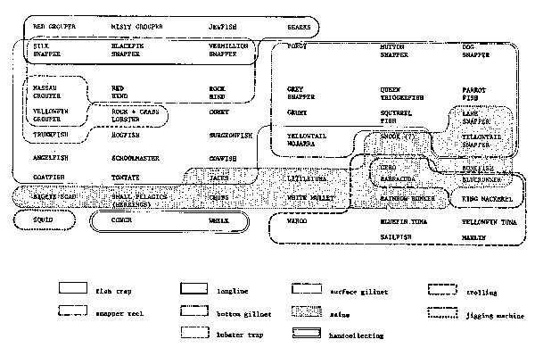
Fig. 3. Species classified by availability to gear, (From Caddy 1983).
Table 2: Methods, utility and data sampling characteristics
for population discrimination.
| Technique | Method | Relative unit cost | Data Type | Determination of population characteristics | Definitive or not in discrimination | Weaknesses and Strengths | |
|---|---|---|---|---|---|---|---|
| A1Protein characterization | a. electrophoresis | low | non-parametric | sample size dependent | yes | sampling difficult | genetic basis |
| b. electrofocusing | high | non-parametric | sample size dependent | yes | procedure slow | highest resolution | |
| c. purification and functional analysis | very high | parametric | sample size dependent | can be | technique difficult | great sensitivity | |
| A2Chromsomal comparisons | a. karyotyping | low | subjective | can be useful | can be differences | requires big | genetic basis |
| b. banding studies | moderate | subjective | can be useful | yes | requires large chromosomes | genetic basis | |
| A3Mitochondrial DNA | a. isolation and fractionation | moderate | non-parametric | sample size dependent | can be for familial studies or dif- ferentiation by area | tedious procedures inherited | maternally |
| A4Color patterns | a. pigmentation patterns | low | non-parametric | can be useful | can be | basis needs determined i.e. ontogenetic or hereditary | usually genetic basis |
| A5Immunology | a. tissue typing, i.e. blood | low | non-parametric | sample size dependent | yes | sensitive to ambient | genetic basis |
| b. microcomplement fixation | moderate | non-parametric | too sensitive | yes | very sensitive | species level tool | |
| A6Numerical or Metrification studies | a. hard part dimensions | low | parametric | can be useful | yes | basis needs determined samples must have common expectation | usually regionally specific, often genetic basis |
| b. morphometrics of body dimensions | low | parametric | can be useful | can be | |||
| B1Growth and life history | a. age-growth by | can be high | parametric | ||||
| dparameters | 1. annual ring on hard parts. | often useful | corroborative | subjective | ease of collection | ||
| 2. daily growth rate | high | parametric | definitive | can be useful | needs calibration | gives rates on short term basis | |
| 3. tagging- recovery | high | estimation | not usually | corroborative | usually biases in release and capture | tagging changes natural patterns on short term | |
| b. onset of maturity | low | parametric | useful | corroborative | differences can be induced by environ- mental changes, | helpful in assessing changes - often | |
| c. fecundity | moderate | parametric | useful | corroborative | difficult to evaluate true number of eggs produced or hatched | less important than the knowledge of where eggs are successful | |
| B2Distribution studies | a. mark and recapture | high | point A to B | can be useful | corroborative | needs substantive | fraught with |
| 1. tags and markers | support data of A type | estimation errors but useful | |||||
| 2. hooks | low | point A to B | can be useful | corroborative | for assessing movements | ||
| B3Natural tags | a. parasites | moderate | non-parametric | can be useful | corroborative | can be lost or | area/host specific |
| b. chemical/hard parts | high | parametric | can be useful | corroborative | transferred can be transferred or source can be spuriously distributed i.e. currents | high information if source specifically located | |
| B4Meristic counts | c. gillrakers or vertebrae | moderate | parametric | not useful in tunas | no | highly variable in some species due to ambient | can indicate some species differences. |
Applications of Stock Concepts and the Underlying Causality Problem
The simple panmixis hypothesis, welded together with the assumption of constant or average parameters in fishery models has led to the long-term failure of “conventional” fishery stock assessment and management procedures in many species, including tunas, and has retarded applied ecology in general. The common denominator is a logical error inherent to the assumed simple stock hypothesis.
“Use of average parameters is non-conservative during times of population stress”.
Although a mathematical average will always be obtainable from a sample, that “average” individual or condition may not exist at any specific moment. This is the essence of the problems with application of mathematical theory and the theories of population genetics, evolution, and ecology as a subset of general biological science. Also there are few environmental characteristics which can be shown to be constant, or near “average” more than two short periods every year or so.
“Evolution of individuals, species and systems are continuous, i.e. progressive.”
As a starting point in delineating “stocks” it should be obvious that the geographic location of reproduction is an important criterion, but that species may have variable geographic and temporally stratified reproduction, sustaining more complex rather than simple panmictic populations within any geographic context. These complex age-structures imply complex temporal and spatial patterns of reproduction.
The recent advances in thinking regarding marine teleost larval fish requirements (Hunter, 1980; Lasker, 1975; Sharp, 1981a, 1981b) have provided considerable basis for changing the usual premises applied to fish reproductive success. The concept of a “survival window” in time and space, arising from studies of the critical energetic requirements of larval fishes and the processes which promote them, is the key to better understanding the multiple cohorts of recruits entering most fisheries.
If we start with the basic premise that it takes nutrients to sustain marine life, and “new” nutrients to either sustain or increase biomass, then clearly one needs to examine the basis of nutrient sources and their availability to larval fishes, and their eventual conversion to biomass in various forms. These are processes determined by energy input and form, i.e. light, turbulence, terrigenic and biogenic nutrients, etc. Starting with photosynthesis, by definition driven by light, the presence of nutrients, and catalysts in the form of organisms, it provides the initial hierarchic step in a long chain of energy transfer and transformation leading up to fishable resources. The larvae must be placed into the appropriate milieu (Sharp, 1981a, 1981b). Until they transform into mobile post-larval stages they are directly influenced by local physical and density dependent requirements in regard to their food sources.
The necessary conditions are not universally or evenly distributed so that each larval group or “cohort” is the evidence for a “survival window” which generated the opportunity for their successful development. That proportion of eggs sown into the sea which will encounter the appropriate conditions, i.e. high food availability and low predator abundance, must be highly variable and likely accounts for the absence of a clear relation between adult biomass and subsequent recruitment in most fishes, but particularly in the nomadic species such as tunas and other oceanic species.
The numerous species of scombrids and their diverse distributions is a clear indication of the complexity of their habitats. The evidence from even cosmopolitan species, like yellowfin and skipjack tuna, supports a localization and differentiation hypothesis for population structures (Sharp, 1983; Richardson, in press). The relative amounts of mixing of population components in various regions very likely accounts for the differences in relative abundance and productivity among regions, and in seasonal and annual patterns of vulnerability to various forms of fishing. Many species are fished during or just prior to their reproduction aggregation. In these instances stock structure studies may be unimportant. However, many species have less well defined reproductive behaviour, and better understanding is required.
The problems of oceanic species compared with neritic species are worth considering before proceeding on to techniques for discriminating populations. For example, the major difficulty with obtaining any rigorous kind of stock identification of or labelling device for tunas is the very cryptic nature of their reproduction. For most tunas we have little or no knowledge of the relation between those individuals recruited to the various fisheries, the adults in major ocean areas and the eggs, larvae and prerecruitment juveniles.
So far in the world's tuna fisheries we have only a few examples where less than 40 cm (or 9–12 month) fish are abundant in commercial catches. The Philippine payao fisheries yield abundances of small skipjack, yellowfin tuna and occasional bigeye, as do the surface fisheries for tunas in the Gulf of Guinea and West Africa. Occasionally similar phenomena are observed in the transition zones in the eastern Pacific Ocean fisheries.
Although there is little evidence for or against localization or very small population ranges in the genus Thunnus, or for the Thunnini in general, it is likely that the smaller, less mobile stages are indeed more influenced by “local”, i.e. metre to kilometre scale, current or water mass phenomena, whereas the 10 cm and greater stages become more and more independent of these “local” features of turbulence, eddies and advection (Sharp, 1981b).
Nakamura (1969) published his anecdotal correlations between apparent abundance, as measured primarily by longline catch and effort, and the current and/or water mass structures. Given this basis, in light of the studies of Saito (1973; 1975) Hanamoto (1975) and Suzuki and Kume (1982), as well as the improved understanding about the physiological ecology of tunas (Sharp and Dizon, 1978; Sund et al., 1981) it is moot that the physical environment heirarchically molds or forms the potential for all fisheries, particularly tuna fisheries. These processes are neither mystical nor particularly untenable, given that one does not expect to predict, sensu strictu, the presence and abundance of fishes in the ocean. The manifold solutions to environmental and ecological challenges to biological persistence are met in the sea by the behavioural and physiological plasticity within and among species.
Except for a few areas, the year to year catch variations for tropical tunas are on the order of 1 to 5 times, low to high, with smaller geographic reference areas exhibiting variations of the order of 20 x, or more (Sharp, 1981b). The relative independence of the larger tunas from local ambient conditions due to their high mobilities can be used to explain some of this variation, the rest is tied up in population structure, component mixing and density dependent schooling dynamics (Sharp, 1978; Sharp MS - What is a tuna school?). To ignore these processes is to ignore the basic tenets of biology, and evolutionary processes.
Other species, as are documented throughout this consultation undergo similar and even greater year to year abundance changes.
To expect less than continuous, slow changes in ecological systems is to be unaware of normal system variations in both ambient energy-nutrient fluxes and subsequent biological responses. These happen on both long and short time scales, affecting local and wider areas. Stock assessment in most cases is still based upon equilibrium states which are not only unlikely, but also misleading. The stock concepts have evolved around this equilibrium assumption and can hardly cope with the processes evident in today's fisheries, i.e., the numerous blooms and recolonizations by species for which we have records of previous fisheries, or the new development of fisheries in areas where these have not been observed before.
In fisheries where fleets are mobile and catch variations are minimal, there is an inherent urge to assume stability of the underlying resource, i.e. unit stock. What this can often be attributed to is that the “stability” is an artifact of “too broad” a definition of the unit stock. In fact the underlying genetic units may indeed be sequentially decimated, without signals from the catch statistics.
Given that speciation is an extreme form of population differentiation in response to environmental changes, the lesser scales of changes and characterization of these processes within a species needs to be understood before a useful stock concept can be clearly defined.
Population Variation and Characterization
The individuals of a given species are the fundamental units of biological evolu- tionarily significant selection. The low fecundity species such as mammals have little chance of having identity in chromosomal-gene level structures, or their expressions. This, and the effects of differing environments produces the nearly infinite array of effects and characteristics in even closely related individuals. Fishes, with superior fecundities, and facing quite extreme selection, have evolved a more near uniformity in many cases, but individuals are still usually distinguishable, if enough characteristics are examined.
The most recent survey methodologies applied to characterization of the genetics of species, which are considered to be relatively sensitive, hence definitive, are:
A 1. Protein or enzyme characteristics
2. Chromosomal comparisons
3. Mitochondrial DNA comparisons
4. Color patterns
5. Immunological reactions
6. Numerical or metrification studies
Methods 1, 3, and 5 are quite discrete and can be categorized as being useful for both differentiation and consolidation of identities. Methods 2, 4, and 6 are fraught with subjectivity and integrative, hence less definitive, except for differentiation, where they are adequate inferential tools.
Another list of inferential tools can be constructed which permit various levels of inference to be made, but which alone cannot be definitive. Unless far more data are collected or spawning populations and/or heritability are known and studied extensively, their uses are primarily for estimation, but all population structure conclusions based only on these data are tenuous.
B. 1. Growth and life history parameters
2. Distribution studies through mark and recapture
3. Natural tags
4. Meristic counts
Because this important domain of knowledge is often only partially available to classical fishery biologists, a short series of discussions of each kind of data is given in the Annex 1 on stock characterization.
Catch per Unit of Effort and Abundance
Effort distribution in relation to the resource distribution, availability and vulnerability needs to be carefully evaluated before fishery data are informative, i.e. interpretable. This usually implies that fishery independent sampling has been initiated (e.g. research programmes or fishery monitoring programmes). The difficulty is to know the true distribution of the resource population, and monitoring this single parameter may tell more about the status of resources than most other statistics.
The first of many sampling problems in fishery research is, therefore, to determine the distribution properties of the subject resource. The aggregations of resources in marine environment are complicated by the three dimensional, highly dynamic transport properties of the water column, seasonal distribution discontinuities and the behaviour of the size-age groups in a population. If the “recruits” to a fishery school, or the aggregate for spawning are diffuse, yet contagiously distributed, sampling inter- pretations change. Of course, the vulnerability of fish, particularly schooling fishes, can vary tremendously in time and space, in response to numerous variables. Since this is the case, tremendous biases can and do result from fisheries sampling these populations. To try to portray the numerous variables in this complex of interactions it should first be recognized that there is a distinction between available resources and vulnerable resources.
The available resource comprises the whole, finite, abundance of the resource, including all recruited individuals. The space frame of the available resource is the total area or volume inhabited by the resource. Depending on the distribution and migration pattern of the subject species and the space constraints of the fisheries, we may find that only a portion of the available resource will occur within the range of the commercial fleet or gear being used. The combination of these two characteristics will define the accessibility of the resource to the given fisheries. Furthermore, only part of the individuals will be vulnerable to specific fishing gear, and will be subject to being caught, either because they are found in relatively big schools, are ready to bite, or show low mobility. For instance, most neritic fishes will be accessible to almost any type of pelagic fisheries provided they are reasonably close to the surface and within reasonable navigational distance from a fishing port, but they will only be vulnerable to purse seine fishing if they are part of a commercial size school. In the simple catch equation
C = qf  (1)
(1)
q is the purveyor of this information. This coefficient can be broken into gear (man), behavioural (biological) and physical (environmental) components which yield perhaps the most dynamic aspects of this simple view (equation 1) of how fisheries operate. Whereas in the past the catchability coefficient (q) has been held “constant” in deference to the nearly measurable C and f parameters so as to determine P; in a number of cases it has become clear that this “convenient” approach can lead to erroneous interpretations (Garrod, 1964; Paloheimo and Dickie, 1964; Clark, 1974; Pope and Garrod, 1975; Francis 1977; Sharp, 1976, 1978, 1979; Clark and Mangel, 1979; Csirke, 1980; Pope, 1980) and a non-useful approach as to the evaluation of the dynamic aspects of both fisheries and schooling resource populations.
While it is fascinating to consider the variability of each of the coefficients in the simple catch equation, it is more important to consider the sources of the variation. What is measured in a typical fishery is the total catch (C) and the fishing effort (f). The total catch has errors in the 5–20% range depending on reporting, species identifica- tion, and proportion of the fish entering controlled markets and fishing effort, has all the associated uncertainties of the catch composition plus a number of other sources of errors related to changes in efficiency, technological improvements, learning changes in target species, etc., which vary widely from one fishery to another.
A list of the variables contributing to C as implied from the three variables q, f and P are given below with contributing variable properties following each parameter.
P, population size, is characterized by
1. Age structure
2. Geographic distribution by size-age
3. Differential ecological interactions by size-age
4. Differential potential for reproduction by size-age
f, the effective effort varies with:
1. Gear type (hooks/day; bait utilized; mesh size; etc.)
2. Relative efficiency (functions of saturation, effectiveness, etc., position
on learning curve of gear, competition or interference of effort, etc.)
3. Distribution of effort over the resource range
q, the catchability coefficient is a “fudge factor” affected by:
1. Availability (function of P2 and P3)
2. Vulnerability (function of biological properties and ambient properties
in relation to f1 and f2)
The biological properties having a direct impact on CPUE as a measure of
abundance are:
a) schooling or aggregating behaviour
b) willingness to “bite” bait or to “stay put” for gear effectiveness
c) seasonal density dependence of P2
The ambient properties affecting CPUE are:
a) sea state, visibility of cues, gear appropriateness, which affects
vulnerability of fish
b) depth of limiting features, i.e. thermal, oxygen profiles, bottom
topography, etc., which affects habitat size of the available resource and
c) proportion of local population drawn or concentrated into area where
fishery is located, i.e. accessibility
Until most properties of these parameters are understood, we will not have enough understanding to explain the variations in catch, relative to effort or any other parameters with sufficient confidence to consider the standard management options a variable resource will offer.
The environmental dependences of variations in q are quite well evidenced in the tuna fisheries of the world. A complete description exists for surface gears, particularly purse seine operations on “school fish” (Sharp, 1978, 1979). Francis (1977) examined q variation in the eastern Pacific Ocean yellowfin purse seine fishery with respect to size recruitment period (semestral groups), geography (nearshore to offshore) for “average” annual data. His table 2 (page 241) shows that there are marked differences between “catchabilities” of tunas by size in the three areas, up to 20 times the “average” annual data. Geven this “smoothing procedure” one could expect at least five times this variation in the individual area annual values, and perhaps several orders of magnitude more from monthly, inter-annual evaluations. Total catch varies on the order of percentages from year to year, local catch varies by orders of magnitude from year to year. Fishing effort varies only in quality and location. This is not unique, but an example of the variations to be expected in schooling fishes.
It appears that many of the problems inherent to the interpretation of fishery data are the result of extrapolation and integration of data beyond their limits of representation. Assumptions are necessary, but their appropriateness, rather than their convenience should be the first consideration. Clearly fishing effort on schooling species is operational only because the fish aggregate. These aggregations have finite distribu- tions or ranges, which vary considerably among species and size age groupings within species. The units of effort are simple predator analogues, which are effective only when a school or an aggregation of schools is behaving appropriately so as to become vulnerable to the gear employed. These schools are not the basic units of the under- lying population in most cases, but composites of what are described as core units (Sharp, 1978) or elementary populations (Lebedev, 1970). The study of the properties of these fundamental building blocks which must converge, merge and redistribute themselves to varying degrees is not part of the “conventional wisdom” of population dynamics, but some believe it holds the key to many important questions.
Clark and Mangel (1979) have given a preliminary description of the Michaelis-Menten, enzyme-substrate analogue models which we feel best represents the important “schooling” dynamics. Their proposed models have definite limitations in application, due primarily to our ignorance of the effects of 1) density dependent schooling dynamics, 2) distances over which the attractions between aggregators and schools operate, (3) size specific behaviour of schooling fishes with respect to same species and multispecies aggregations and 4) the distribution properties of the size similar, core schools which are the building blocks of the underlying population fished by the various gears. The important questions are the dynamic ones, but a fundamental basis for our understanding of these depends more on the validity of the “core school” concept.
Fishes with some dispersion in their occurrences provide even more intriguing problems, particularly if their habitat of life history includes a gradient in vulnerabil- ity and a substantial portion of the resource can be considered to have a “refuge” against fishing effort, i.e., Trachurus species in the Eastern Boundary Currents, some flatfishes, oceanic species, etc. Other examples are species associated with kelp beds or rock piles, where usual trawling effort is not effective or practical. What is needed is some estimate of “recruitment” to and from the refuge. The problem is that sampling and monitoring is far more complex than a “normal” fishery sampling programme can provide for, hence we can lose track of substantial population elements. This phenomenon could account for a large amount of unexplained “stability” of some resources in the face of intense exploitation.
Fishery resources can be found in innumerable distribution patterns, from windrows (i.e. invertebrates) to schools on through relatively uniform dispersion over a habitat. It does not matter so much which pattern is prevalent, as long as it is known to some degree. Schooling fishes are often aggregated in density dependent, size (length) determined groups, usually with a negative binomial aggregate-size frequency. Fisheries select for intermediate to large schools for obvious reasons, and this confounds interpretation of catch and effort related statistics. The distribution frequencies of individual schools would better reflect local abundance of density than the integral catch rate statistics, except when a resource is very disperse (i.e. not aggregated). Only careful records of time and space related catches (e.g. via precise logbook reports) can help one interpret such interactions.
Causality and Hypotheses Structuring in Larval Survival
Continuous studies have sought to close one of the most important gaps in fishery science, the one which stands between a cohort of fertilized eggs' entry into the sea and the recruitment of the subsequent group of fish at some later date to fisheries. The problem hinges around the observation that some 5 to 6 orders of magnitude losses are realized during this period, and usually estimates of year to year recruitment variation for natural, not heavily exploited fish populations range from about 2 or 3 × to about 500 × or about 2.5 orders of magnitude (Ursin, 1982; Hennemuth, Palmer, and Brown, 1980). Ursin's (1982) discussion of the relative stability of ecosystems suggests that even this variation is small compared to what might be expected unless there are considerable stabilizing influences.
Rosenthal (1970), Jones (1973) and Lasker (1975; 1978) have each rediscovered the early life history as the most sensitive period, as proposed by John Hjort in 1913–1914. The modelling studies of Vlymen (1974; 1977), Beyer (1980) and Beyer and Laurence (1981) provoke one to consider that spatial distribution and quality of esculent particles in nature control the first in a sequence of hierarchic hurdles to be cleared if any larval fish is to survive to reproduction ages (Sharp 1981a).
While theory, modelling and restructuring of research plans and activities have taken some years, recent reports (O'Connell 1980) and research in progress (Theilacker, personal communication) have given adequate support to this concept that to ignore it is futile. Likewise the importance of predation cannot be in any way ignored, as clearly natural mortality is either due to direct or secondary predation (M = Mp1 + Mp2). The problems of monitoring directly either Mp1 or Mp2 are formidable, and to-date are not well documented for larval fishes in nature except by inference (Alvariño 1980). Sampling post-larval pelagic fishes is sufficiently difficult that quantitative studies of distributions and abundances are nearly non-existent. Demersal post-larvae of some species are somewhat less difficult to sample, and Zijlstra, Dapper and Witte (1982) offer again remarkable insights into variations in growth, mortality and early life history related density dependent processes for one demersal species.
Meanwhile other researchers (Owen 1981, Mackas and Boyd, 1979; Sameoto 1981, Smith et al., 1981, and Coombs et al., this volume) are finding that the stratification and densities of organisms, larval fish food particles and larval fishes are indeed related on scales predictable from models and laboratory physiology and behaviour studies. These studies are the necessary logical feedback into the restructuring of research programmes and continue to add fuel to the efforts of climate-ocean researchers to find linked cause- and-effect relations between climate-weather-ocean variability and subsequent larval and small juvenile fish survival (Bakun and Parrish 1981, Bakun et al., 1982, Parrish et al., this volume).
Platt and Denman (1975) have given a fair representation of the expected biomass spectrum (particle size frequency), and a good example of a “bolus” of energy passing upward through this spectrum. The point that needs considered is that the distribution of volume densities (contagion) are greatly affected by the negative binomial distribution at each and any size range, i.e. it takes several orders of magnitude more individuals of 50–200 ymx phytoplankters to reach a mass equivalent of even a fish larva, but we only rarely observe via sampling naturally occurring densities of phytoplankters of this size range in sufficent relative abundance or concentration to support feeding fish larvae (e.g. 0.8 to 3.0 times the larval fish biomass per day, depending upon species, temperature, and activity of the larva).
The concept which is often neglected is that where the lower densities prevail, none of the predators in the milieu can operate in a positive energy balance. This leads one to reason that larger individuals need to be mobile in order to survive, and that the smaller predators, i.e. fish larvae, must either be situated in or very near appropriate densities or they will indeed starve, and become subject to predation (Sharp 1981b).
Simpler, single cell organisms have evolved stasis mechanisms such as encystment and dormant phases which preadapt them to nutrient poverty periods of relatively long duration. Settling out of the upper water column, into cooler waters, slows basic metabolism to some degree, but to be successful, i.e. persist and reproduce, single cell organisms or small predators must either be transported or swim upward into photic, productive waters again, or be able to somehow persist on the rain of detritus and debilitated organisms from above. Those that cannot will themselves become detritus.
Since it is also certain that nutrient and particle injection into the photic zone that is sufficient to stimulate primary productivity is neither uniformly nor stochastically distributed in regard to location, timing or amount, then it is nearly certain that the sequential processes of colonization, predation, growth and reproduction by each oviparous fish species contains a series of low frequency-of-occurrence requirements which cannot be attributed a priori probabilities or even averages. Hence stochastic, process models might only be useful to represent known distributions and occurrences. This also implies that only causal ecological modelling based on directly linked processes or localized interactions can be expected to be predictive in any realistic sense. Probabilities of interaction are therefore, only interesting on very small scales, i.e., meters/minutes (see Vlymen 1977), whereas above these scales they approach zero very rapidly. The only reprieve in this case is the increased mobility of larger predators which expands the probabilities of interactions over larger scales, i.e., km-days, between larval fishes and their more mobile predators. However, as the larvae develop, their numbers decrease and even though total biomass goes up, their tendency to aggregate also increases, decreasing a predator's opportunity to encounter them. (Further evidence that this is a problem is the fact that the first schooling phases and their predators are poorly known for most marine fishes due to their infrequent occurrences and patchy distributions (Hewitt 1982, Smith et al., this volume). This decimation and biomass increase is an ever upward spiralling continuum which ultimately results in the various observed distribution patterns and characteristics of adult fishery resources, i.e. solitary to schooling, sedentary to highly mobile; abundant to rare; small size to larger size; homing reproduction to opportunistic reproduction; wide distributions; or limited distributions. What is important is that the eggs be placed into sufficiently amicable environments to begin development; that upon hatching they find themselves in the “rare” high density portion of the distributions of their food; that they find themselves in a null or near null abundance of their respective predators; and that they manage to develop rapidly enough to mobile stages, perhaps even to schooling stages, so that they can begin searching for the even rarer abundance distributions of their, now somewhat larger prey.
The picture culminates in the simple realization that the distributions of all the lower trophic components are discontinuous, that these species are characteristically opportunists with high production rates, and that these species have evolved in harmony with discontinuities in the physical environment which promote their regular, i.e. serial bursts of productivity, hence persistence.
It is certain that monitoring only larval fish distributions and food particle stratification/destratification processes will not be adequate to allow complete explanations of recruitment in any “larger” system today. However, it is also certain that unless these basic measurements are included in the data proposed to monitor or explain recruitment, there can be no progress. The predator-prey research and technology for sampling post-larval and juvenile fishes up through about 5–20 cm lengths needs a lot of improvement before the complete logical bridge is made between eggs and recruits to fisheries. Methods for measuring organism size distributions in relatively large volumes of open ocean need to be developed so that eventually any major effects of harvests by man or major predation might be measured. It appears that in spite of our zealous efforts to understand the spectrum of fishery resources above “recruitment” sizes, the most biologically important and dynamic changes all occur well below this threshold, while these changes may well be influenced by climate-ocean phenomena many thousands of kilometres and months to years away.
Preconceived Results In Stock-Recruitment Relationships
Perhaps the most common difficulty in which fisheries scientists find themselves when trying to apply their knowledge to fishery data, in contexts of available tools and methodologies, is how much data can or should be “averaged” or integrated to adequately represent a resource. For example, the simple portrayal of Population Fecundity (viable egg production) in any given year and potential recruitment resulting sometime later usually takes the form of a table of figures as shown below:
| Year | Estimated total eggs produced | Resulting recruits in year (+n) |
|---|---|---|
| tX | 14 × 1013 | 8.6 × 10⁶ |
| tY | 15.5 × 10¹³ | 6.0 × 10⁶ |
| tZ | 22 × 1013 | 10.2 × 10⁶ |
| . | . | . |
| . | . | . |
| . | . | . |
| tN | i | j |
A simple plot of j against i for a sequence of years is the usual end point. Some assumptions about a model/form are made and some sort of estimate of the relation between the two estimates is produced. Even less elegant is the use of biomass of adults in the place of total population fecundity, as integrated by use of the biomass figures.
Recent insights about engraulid populations and sequential or iteroparous reproduction shows that for some populations a biomass estimate cannot really be used by itself as an estimate of recruitment potential (Hunter and Goldberg 1980, Parker 1980, Hunter and Macewicz 1980, Alheit et al., this volume). Except for a few “homing” populations with precisely determined reproduction periods, it is most that such attempts to portray potential recruitment are futile exercises.
However, another question can be answered from estimates of egg abundances in the sea. The question is what is the minimum biomass of the females producing the eggs observed? If the data are collected over sufficiently extensive time-area strata to extend beyond the range of reproduction, and if the population is somewhat conservative in its reproduction behaviour, i.e. not too large a variance in either proportions of females spawning, or eggs produced per female biomass, then a reasonable and useful estimate of spawning biomass can be made (Alheit et al.; Smith et al.; Watanabe; all this volume). It is quite a bit less complex to make these calculations for species with either direct (linear) relations between size-age and eggs produced than it is for a population with allometric fecundity and many size-age classes.
On the other hand, knowledge of only the eggs produced will not result in a reasonable “prediction” of the amount of recruits. It is the sequence of events beyond the egg's production and release into the sea which determine this, and these are not events which are uniformly or stochastically occurring (see Kawai and Isibasi, this volume).
The examples provided by Shelton and Armstrong (this volume) on both the anchovy, Engraulis capensis and the pilchard, Sardinops ocellata, from two fisheries (South Africa and Namibia /Southwest Africa) can be useful in illustrating some of the questions we are trying to address. Figures 4 and 5 show for the pilchard the annual figures for potential spawning biomass and subsequent recruitment. By connecting segmented points starting with the earliest years for which both estimates are available, we have a new insight into the recruitment story. The longest series is that for the South African fishery (1950–1982). The 1950 through 1954 points are clustered about 500–750, 000 ton spawning biomass and recruitments are estimated to have been over the range from 8 to 16 × 109 individuals. Comparable recruitments occur for the years 1971, 1973, 1974, 1975, 1967 and 1968 when spawning biomasses were relatively stable at about 100, 000 tons. Of greatest interest, of course, are the years 1955 to 1962 when the recruitment and subsequent adult biomass bloomed. The surges of recruitment in 1955 to 1957 lead to the adult abundance increases in 1958, 1959 and the 1960 peak of over 1,400,000 tons. Subsequent to 1960 there was a steady decline in both adult abundance and recruitment. While in fact only 1962 recruitment falls within the range of the 1950 to 1954 levels, and from 1963 to 1966 recruitment was quite low but stable, i.e. on a parr with recruitment observed since 1976.
This suggests that the system controlling recruitment went through a sequence of state changes, the earliest ones 1955 to 1957; 1958 to 1960; and 1961 to 1965 where the population size changed dramatically in response to several variables: 1) recruitment enhancement, 2) declining but large recruitment and increased abundance of older age classes due to the previous recruitment, and 3) decreased recruitment as well as senescence and fishing induced biomass declines. Since 1966 the population is small, relatively stable, and the responses of recruitment are obvious. However, the most interesting message in this series is the relatively ‘stable’ recruitment since 1962–1963. This feature implies that there are “other” limitations on recruitment beyond biomass of spawners.
The sequence of information on the Namibia - Southwest African pilchard fishery is shorter, 1970 to present, but can be contrasted to the situation described in the South African fishery. It would be better if a longer time series were available, but the catch records clearly indicate a northward shift of the abundance of pilchard in response to the massive growth of the population of South African pilchard in 1958–1959. The catches of pilchard peaked in the north in 1968, while the catches were returning to pre-bloom levels (pre-1958) in the south. Clearly the sequence (1970 to present) portrayed in Figure 4 is only part of a complex story in which the sequence preceding it must also have been analogous to that in Figure 3 with a recruitment bloom starting in about 1964–1965, ending in 1967 or 1968 and then arriving at the lower 1970 series of Figure 3.
This set of scenarios compells one to consider that the system-wide patterns of recruitment, from setting adjacent geographic bits together in temporal sequence, to be perhaps the following:
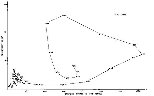
Fig. 4. The South African pilchard recruitment-spawning biomas data from Shelton and Armstrong (this volume) with the fitted curves removed can be quite informative if arrayed in sequence. Note that the entire fishery from 1955 to 1962, 1971, 1973–1975 and 1967–1968. Poor recruitment does not appear related to spawning biomass, although that biomass certainly reflected previous recruitment success.
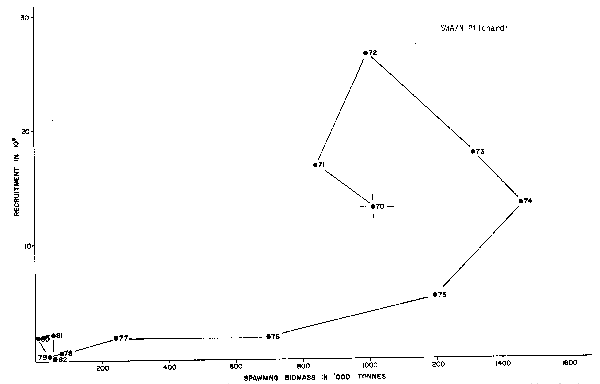
Fig. 5. The Southwest Africa/Namibia pilchard data on recruitment-spawning biomass (from Shelton and Armstron, this volume) shows a similar spiraling diminish. There is a clear indication that the population density-center changed in the sardine fishery during the years 1960 to 1970, with recent years in both fishing areas being poor since 1975 (see Figure 4 and next).
The anchovy examples are shown in Figures 6 and 7. The South African anchovy population shows a series of bloom and recession cycles in the period from 1964 to present. A minor bloom is evidenced in 1966 to 1967, a major bloom occurred in 1973, then a series of years of relative stability are observed from 1975 to 1980. In 1982 another major bloom is indicated. All of this is in the face of increased fishery removals.
The Namibia/Southwest African population information sequence is again very short, i.e. 1972 to present, making it difficult to compare directly with the South African information. However, the recruitment has been relatively stable between about 55 and 75 × 109 individuals per year over a range of about 100 to 340,000 tons of spawners, with a trend in low years (1976, 1977 and 1979) where lower biomasses yield lower recruitment. In direct contrast with the South African situation, 1982 recruitment is estimated to be very low. Both data sets imply little relationship between adult biomass and recruitment enhancement.
Another useful data series is that from Watanabe (this volume) where he explores the relations between eggs produced in each year, and the eggs subsequently produced by the progeny of that year. Figure 8 shows this pattern for the sequence of years 1951 to 1976 for the common mackerel (Scomber japonicus) population of the northwest Pacific. Note the sequences of cyclic blooms and recessions commenced with a bloom observed in the years 1951 through 1963. The first collapse cycle begins in 1964 and by 1968 is complete. The subsequent bloom starts in 1969, from a relatively low production of 200 × 1012 eggs, rising steeply in 1970 and 1971 from similar egg production until recruitment to the spawners ensues in 1972 through 1976. The decline in egg production, hence potential recruits begins in 1974 and continues despite high egg production through the end of the series, in 1976.
This double cycle of bloom and recession shows, once again, an independence of implied causality between eggs that generate a given year class and subsequent eggs produced by that year class and in fact shows that these are two periods with entirely unrelated abundance cycles which are more likely due to changes in ambient conditions and distribution than to adult abundance, per se. A feature already demonstrated to be a major cause of variability of recruitment in the Peruvian anchovy by Csirke (1980).
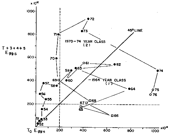
Fig. 8. The data on egg production in any year versus eggs produced by the progeny of those year classes (from Watanabe, this volume) shows a series of complex bloom and recession periods for Scomber around Japan. The importance of sequential year class survival and subsequent egg production cannot be ignored, but fitting lines through each time series (i.e. period 1) 1953 to 1964, or 2) 1969 to 1974) does not help one understand or imply any stock-recruitment relation.
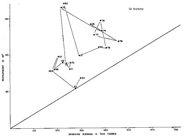
Fig. 6. The South African anchovy recruitment-spawning biomass data (from Shelton and Armstrong, this volume) indicate that this resource is still in a positive state with respect to recruitment. The spurt of recruitment success in 1973 resulted in a biomass increase which was sustained up through 1980, but the lower recruitment from 1979 to 1981 tended to shift the biomass back toward earlier levels until the 1982 bloom.
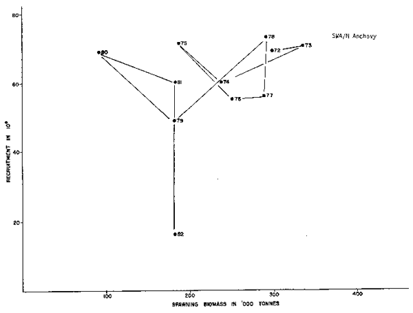
Fig. 7. The Southwest Africa/Namibia anchovy situation with respect to recruitment appears rather constant up until 1982.
Watanabe (this volume) also presents similar data for the shorter time series, 1960- 1978, for Sardinops melanosticta. There are two short cycles again indicated with a low period of abundance from 1960 which subsequently declines to unestimably low levels until about 1970, when a new “abundance” cycle began, attaining the heights described in various reports (Tanaka; Hiyashi; and Kawai and Isibasi; all this volume). The egg production cycle began declining again in 1976, and will be an interesting feature to monitor, as suggested by Watanabe (this volume), as an indicator of future stock potential, but not predictive until the recruitment and mature stock abundance is obvious from other measures (Figure 9).
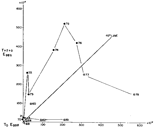
Fig. 9. Similar egg to egg production data for the Japanese sardine (from Watanabe, this volume) shows once again the futility of fitting “mean” stock- recruitment lines to such data. Clearly any implied relation severely over- estimates the likely recruitment or egg production for poor years while a time sequence plot can yield useful insights into likely trends.
The value of this approach is that clear indications of changes in system state are evidenced, lower abundance bounds are made more obvious, and declines are signalled, indicating periods when care should be taken and monitoring of other indicators such as age structure, distribution and abundance blooms of predators should be more closely monitored.
A series of abundance-increase data (which normally compares increased recruitment, increased catches, increased fishing effort, etc.) can easily generate a done shape curve with a form resembling some presumed stock-recruitment curve, a yield per recruit curve, and even a surplus production curve, all depending on what is the source of the basic data and mostly on what interpretation is being given to it. Fitting a model can therefore be purely artefactual and will normally tend to give the wrong answer to key questions such as: 1) What spawning population abundance will provide for persistent, relatively high potential reproduction? 2) What is the lower level of population which can be expected to support a substantial bloom given the appropriate conditions?
This latter question is posed only by considering these observations and concluding that the bloom cycles are stimulated by non-fishery related phenomena, and are relatively short term. The subsequent increases in distribution and overall abundance, each act to increase potential reproduction, although not necessarily determine their realization. The collapse cycles, on the other hand, do indeed reflect major components of causality in some studies (Csirke 1980; Santander et al., this volume) and warrant further investigation of such features as cannibalism, disease and other density dependent phenomena.
CONCLUSION: WHY MODEL FISHERIES?
In the absence of clear objectives for fishery and fishery related ocean science, there have been significant changes in general attitudes about what these objectives might be. Tautological dialectics about promoting stable fishery production and maintaining species in perpetuity, etc., hardly represent all realistic objectives in the “real-world” of societal demands, growing populations, political economic decisions regarding exploita- tion and distribution of benefits from renewable marine resources, particularly while facing the perpetual climate-ocean variability which affects each of these.
The main biological variables surveyed here will all need to be considered as potentially strong affectors of fishery models. The simplified models which have evolved have had their utility, and certainly, their severe short comings. The problems of population definitions, basic biological units of interest, and their interactions with other ecosystem components, biotic and abiotic, need to be kept in perspective, and resolved to adequate degrees. Adequate, meaning in this case sufficiently well to be useful in forecasting or predictive models. Hindcasting or historical monitoring models can be (and usually are) less rigorous since they are not critical as bases for immediate decision making.
Even with exploitation unit concepts and resource definitions clearly in hand, modelling has yet to evolve toward a level suggesting the reality of the many changing population responses such as those discussed. Changes in: growth rate; natural mortality rates and sources; carrying capacity at all life stages; distribution and relative abundance; hence density at each stage; all affect the future status of any resource. The changes in age structure, available refugia or determinant processes leading to mortality at any life history stage severely influence any potential to resist either natural or man induced perturbations in the ecosystem.
We are not advocating modelling of the Universe, but only that if any resource is truly important that there be given due consideration to the observations that traditional or conventional fishery models have yet to prove adequate, or even appropriate in many cases. There are obvious exceptions, for example the amazingly stable North Sea plaice, upon which many leading fishery scientists have based their enthusiasm for both age structured and production models. But, … it should be kept in mind that only diligence by marine ecologists and oceanographers has kept at least one of the major nursery areas (The Wadden Sea) from joining other “industrial wastelands” and thereby insuring, at least temporarily, a future for this component of the production from the North Sea (See Wadden Sea Working Group Reports 1–11, 1982).
It is likely that specific bivariate plots of each pair of fishery-biological variables will or can hold answers to dynamic fishery questions? Even if the answer is “No” they might and have proved to serve as useful aids in evaluating the appropriateness of many conventional questions. If, no matter how precisely the information gathered, the variables do not give indications of any direct relation, then it is appropriate to declare the question inappropriate, null and void. Reformulation of the question is in order. This is progress. This is what we hoped to achieve during this Consultation.
Other questions needing answers have been discussed here and in other fora (i.e.; Caddy 1983), and two that need particular attention in regard to man's role as major predator are:
If these were well known, it would appear that perhaps managers and decision makers would learn what are appropriate biological questions to ask, and we, as scientists, might be able to formulate and execute research and moritoring schemes to answer them in reasonably synoptic fashion.
Much of marine science can be said to be answering questions for which answers would be nice to know. More important in applied fishery research is that there be more attention paid to formulating answerable questions which need to be known. This is particularly true if we intend to involve other disciplines and fields of interest which have their own immediate problems.
By focussing attention on such phenomena as El Niño, it is possible that there is a misemphasis of important alternative states of the ecosystems involved. Where many are still trying to attribute the demise of the Peruvian anchoveta to the mythical El Niño of 1971–1972, the processes were already well in gear prior to this ‘event’. Glantz (1981) has addressed the societal benefits of an El Niño forecast, and inter- governmental bodies have made efforts to not only define El Niño (SCOR Working Group No. 55) but also now scientists have attempted to discover their underlying causes and predict them. Because of the immediacy of the effects draughts and floods, which are among accompanying symptoms of El Niños, are given more attention. However, the fact that El Niño is not regional, but an oceanwide process has only recently been generally recognized. As yet no one has responded at National levels to the consequences of Guillén's “Anti-El Niño's” on fisheries. Kawasaki (this volume) has provided an interesting correlation between fishery processes across the Pacific Basin which would suggest that modelling and predicting fishery responses has indeed longer term components than only todays fishing effort or todays habitat and ecological status. There is a history and a future which, although they might cycle about some median state, do not permit the broad handed “averaging” of information.
The time to begin facing these problems, reformulating questions and developing new techniques to answer them is now. There is little need for new theory. What is needed is clear headed, pragmatic science of the sort everyone talks about but too few are ready to do, for whatever reasons. The major stumbling blocks to progress usually involve persistent optimism about technological or simple, quick-fix solutions. The solutions lie in hard work at sea, in the laboratory, by innovative multidisciplinary study and gathering of long time series of information, and on a precise knowledge of what are the questions that need answering. The questions needing answers will be posed in a changing societal milieu, and will certainly become more demanding than ever before. If it is recognized that the equilibrium or averaging concepts have proven to hinder rather than help in facing the problem of variations in climate-ocean processes, and their products, fishery potential; and if it is also recognized that the fishery is just one of the many elements to be considered in modelling fisheries, then we may find this to be the age of rediscovery in fishery science.
In the meantime, as fishermen need to fish and resources need to be harvested, sources and patterns of variations should be identified and taken into consideration when interpreting the output of classical models. What is even more important is to evaluate the amount of risk involved by not taking, or not being yet able to take, important externalities into consideration. This will be carefully considered, and any obvious concerns explicitly stated. Until these uncertainties are accounted for it cannot be said that “fishery management” works. It can only be said that there is a lot to be learned before we can be sure we are even approximating adequate monitoring of the complex fishery systems we are charged with sustaining.
ANNEX 1
DISCUSSION OF METHODS OF STOCK CHARACTERIZATION
A1. Protein and enzyme characterizations are possible through a number of techni- ques which range from electrophoresis and histochemical staining techniques, electro- focussing to chemical purification, and thermodynamic-biochemical function studies. The latter types are extremely costly in time and materials, and are usually only effective at species, or in rare cases at sub-specific levels, for identification of sub-population distinctions. The rare cases would include species isolates with clear distinctions and no mixing.
Protein electrophoresis is the presently dominant technique for rigorous population discrimination procedure in studies of avian and terrestrial vertebrate populations with clearly distinctive barriers to interbreeding, even where some parts of life history stages are coexistent. The applications in the marine environment have been of mixed utility primarily due to misjudgement of the nature of intra-species or sub-population differences.
The statistical requirements and sampling strategies are determined by the non- parametric nature of the data due to the discrete nature of the variation, and the behaviours of the species' populations in reproduction. If a species does not “home” or obviously isolate itself at reproduction. or at some opportune moment for sampling then it is very difficult to obtain sufficient evidence to rigorously define population structures. However, far more inferential power is available in the face of even this problem than is available from category B methods, given the same problems of reproduction behaviour.
A2. Chromosomal comparisons are now classic in species such as Drosophila and Chironomids which have few, large and highly structured chromosomes. Fishes do not exhibit obvious stratifications from this perspective as their chromosomes are numerous, small, and not yet well described, except for a few species.
The techniques available for studying chromosomal variation are tedious and time consuming, and non-parametric data results, so that these are not promising in studying any but isolated reproductive groups or known spawning fish. Finding no differences cannot, however, be interpreted as being definitive in species with numerous small chromosomes due to the resolution problems described previously.
A3. Mitochondrial DNA is maternally inherited and could be quite useful in studying relations or affinities within and among schools, as hypothesized to exist within similar size fish within schools (Sharp 1978, 1981b). The technique is recent (Giles et al., 1980; Avise et al., 1979; and Lansman et al., 1978) and is useful for relatively limited and intensive studies until better characterized. The absence of a discrete functional quality or character other than size or weight of DNA fragments makes comparisons essentially one of analogy to meristic measures, although heritability is implied. When possible this should be shown rather than assumed. It will be at least a decade before this technique will be evaluated for utility in discriminating breeding units of oceanic species.
A4. Color pattern and pigmentation studies fall into several categories. Where pigmentation is often a developmental (sequential) process, there are often neotenic arrests, or slow downs in individuals within distinct geographic regions. Atlantic albacore exhibit these processes (Aloncle, personal comm.). Whether these are population characteristics or only developmental anomalies due to environmentally induced processes is not likely to be known until culture and laboratory breeding studies of marine fishes is well advanced. On the other hand Perrin (1975) and Evans (1975) have shown that the study of color patterns are useful genetic tools. At present color patterns appear to have limited potential in this area for most fish species.
A5. Immunology has receded from favor in applied studies since the late 1960's because the results of various studies tended to imply far more complexity than was expected in and among species (Deligny, 1969; Sprague, 1967; and Sprague and Fujino, 1965).
The procedures are not difficult and they are both economical and rapid, but the interpretation of results is tedious, often complicated by the effects of ambient conditions where the immune assays are performed, i.e. temperature, light, contaminant aerosols, etc. If a better controlled environment, a special chamber or other mechanisms could be employed to remove these variables, an at-seas sampling programme could be devised to re-evaluate the utility of this tool.
As in electrophoresis, the data are non-parametric, and therefore sample sizes and sampling strategies would need to be rigorous, and these studies are therefore demanding. Breeding studies would be extremely valuable in conjunction with this approach.
A6. Numerical or metrification analyses, as defined here, are multivariate morphometric and/or growth pattern related studies, as opposed to meristic counts. Numerical techniques comprise primarily tedious multivariate data analysis of suspected related groups, contrasted among themselves in order to determine the affinities or levels of relation. Except in clear-cut divergences, close sub-specific groups are likely to be given greater or lesser affinity than closely related but even obviously different species. Numerically derived cladograms can give very opposite results from those based on clearly defined process-related studies of morphology, genetic characters, and even behavioural information (Sharp and Pirages, 1978; and Le Gall et al., 1976). However, to find clear, slightly or non-overlapped morphological properties among samples of a species with uniform expectation is a powerful inferential tool even if rarely encountered. The key is in the knowledge of when and where to look. For sub-specific groups which poten- tially mix, the sampling problems are formidable. For widely distributed species with simultaneous occurrences at extremes of the species habitat, sampling at these points can yield useful and stimulating sampling insights, particularly if studied concomitantly with other category A and B methods.
B1. Growth rate, respiration and developmental sequence are all population specific properties, with great overlap and graded variation within and among populations. In the nomadic species like the tunas, with their great diversity of environmental options, physiological and behavioural responses are also quite diverse; growth rate and onset of maturity studies are still developing, but there are clear dichotomies arising. The studies of Cayré (1981, 1982) on skipjack behaviour and fecundity in the eastern Atlantic indicate at least two different physiological/behavioural groups are frequently encountered where both differences in fecundity at size and school specific fecundity and ovarian state at size are observed.
The importance of population parameters in characterization of resource parameters is fundamental to evaluation of the fishery potentials of the various populations, but such observations as highlighted by Josse et al. (1981), show the great differences and confounding features of studying opportunist species such as tunas in contrast to localized or homing species (Sharp 1981b).
B2. Mark and recapture studies are good for primarily one definitive aspect of “stock” characterization; fish can be shown to move from the point of receiving the mark to the point of recapture. Other inferences will depend heavily upon other data. Since recapture in most fisheries is dependent upon environmental characteristics and the distributions and kinds of fishing effort, unless the entire habitat is fished, the results are often severely biased, hence of limited value to population structure studies.
The application of mark and recapture experiments in defining “stock structure” depends solely upon the supportive data set accompanying the studies. It has not yet been proven for any fish that tagging alone has had a definitive role in determining stock structure, it is solely an inferential aid. Albacore crossing the North Pacific or a codfish crossing the Atlantic does not prove the single genetic stock hypothesis, or panmixis, it only suggests that some population components are actively making transoceanic crossings. Whether there is a single, simple population or several is only proved through characterization studies based on genetic information, principally from A1, 3 and 5.
B3. Natural tags fall into two types, those obtained from the environment which are permanent and those which can be trasnferred and/or lost. Of the first category we have examples of chemical isotopes which arise from point sources in the environment, and incorporated by individuals either directly from solution in the water column, or by dominant food organism concentration, and assimilation, or both. The studies by Calaprice (1971) and Calaprice et al., (1971) have shown useful examples of this type of natural tag in salmonids species arising from known spawning grounds, with characteristic chemical patterns.
Of the second category there are distinctly conflicting possibilities which confound the interpretation of the results, hence diminishing the utility of the tools. Parasite- specific studies fall into this category. If a parasite is carried specifically by a host with a limited geographic range, delimiting the distribution of that parasite, then the parasite is a good marker or natural tag, comparable to those in category B2 for studying the distribution of the host species arising from the parasite's habitat.
However, if the host or the parasite can be separated (lost) or transferred (by predation of the host) by a species with a broader range, then the utility of the parasite as a definitive label, as contrasted to a “distribution” indicator, is lost too. The use of parasites to determine population structure depends heavily upon supporting information and can be corroborative, but is not alone definitive.
Chemical tags have to be evaluated in the same light as parasite information. If for any reason one suspects that the chemical tag can be lost or transferred, then its utility as a delimiting character is lost.
Natural tags in hard parts can act as records of life history processes. Oxygen isotope ratios can yield information on temperature exposure, and the changes of habitat, i.e., fresh to saline, saline to freshwater, can certainly be observed. Fishes with complex life history patterns in local regions could be studied quite usefully in this regard, while mesopelagics and most tunas, with their subsurface, thermocline centered habitats, prove more of a problem both logically and realistically.
The problem reduces to one of observations on Lagrangian water motion and water mass parcel distributions in the ocean. Rossby, of the Woods Hole Institution of Oceanography, has studied for several years the Lagrangian transport of SOFAR floats through acoustic methods across the North Atlantic from the mouth of the Mediterranean to the west across the Atlantic Ocean, throughout the Sargasso and Gulf Stream related water masses. The complexity is astounding. The upper and lower thermocline transport is relatively independent. Studies of chemical tags could be quite misleading.
B4. Meristic counts, like life history patterns and natural tags are due to local, but short-term exposures, with genetic underpinnings. The causal studies of Lindsay (1961) and Taning (1952) show extreme meristic variation. Differences are primarily dependent upon such variables as temperature exposure and development time. These are neither definitive nor inferential data without several concomitant information sets. For example, if one could use oxygen isotope ratios from chemical tag studies of hard- parts to characterize temperature epochs of early life history stages along with meristic counts, perhaps single populations spread over broad geographic ranges (latitudinal or depth) could be interpreted to comply with a simple stock concept. The important initial data would be category A studies. Without those data the meristic sampling observations could be entirely misleading and illogical bases for drawing conclusions on population structure. Gibbs and Collette (1967) show that meristics are barely useful as species identification tools for the genus Thunnus.
For opportunistic and widely distributed species it is unlikely that any of these data sets (A or B) will, alone, be adequate. Other sets of data which can be useful are length-age frequency data and sex ratio with size. These permit an evaluation of a few behavioural parameters, as yet not given appropriate attention in population studies.
REFERENCES
Aiken, J. 1981. A chlorophyll sensor for automatic, remote, operation in the marine environment. Mar.Ecol.Prog.Ser. 4:235.
Alheit, J., B. Alegre, V.H. Alarcón and B. Macewicz. (This volume). Batch fecundity and spawning frequency of various anchovy (genus: Engraulis) populations from upwelling areas and their use for spawning biomass estimates.
Alvariño, A. 1980. The relation between the distribution of zooplankton predators and anchovy larvae. Calif.Coop.Oceanic Fish.Invest.Rep. XXI:150–160.
Andersen, K.P. and E. Ursin. 1977. A multispecies extension to the Beverton and Holt theory of fishing, with accounts of phosphorus circulation and primary production. Medd.Dan.Fisk. Havunders. N.S. 7:319–435.
Avise, J.C., R.A. Lansman and R.O. Shade. 1979. The use of restriction endonucleases to measure mtDNA sequence relatedness in natural populations. I. Population structure and evolution in the genus Peromyscus. Genetics. 92:279–295.
Bakun, A. and R.H. Parrish. 1981. Environmental inputs to fishery population models for eastern boundary current regions. pp. 67–104. In Workshop on the Effects of Environmental Variation on the Survival of Larval Pelagic Fishes (G.D. Sharp, ed.). IOC Workshop Report No. 28. IOC/UNESCO, Paris.
Bakun, A., J. Beyer, D. Pauly, J.G. Pope and G.D. Sharp. 1982. Ocean sciences in relation to living resources. Canadian J.Fish.Aquat.Sci. 39(7):1059–1070.
Baranov, T.I. 1918. On the question of the biological basis of fisheries. Nauch.issledov.iktiol, Inst.Izv. 1(1):81–128. Izv.ryb.i nauch.issledov. 1(1). Moscow.
Beverton, R.J.H. and S.J. Holt. 1957. On the dynamics of exploited fish populations. Fishery Invest.London. Ser. 2 (19):533 p.
Beyer, J.E. 1976. FISH I. Survival of fish larvae - a single server queue approach. Inst.Math.Stat. Oper.Res., Technical University of Denmark, Lyngby. 244 p.
Beyer, J.E. 1980. Feeding success of clupeoid fish larvae and stochastic thinking. DANA. 1:65– 91.
Beyer, J.E. and G.C. Laurence. 1981. Aspects of stochasticity in modelling growth and survival of clupeoid fish larvae. Rapp.P.-v.Réun.Cons.int.Explor.Mer. 178:17–23.
Booke, H.E. 1981. The conundrum of the stock concept: are nature and nurture definable in fishery science? Canadian J.Fish.Aquat.Sci. 38(12):1479–1480.
Caddy, J.F. 1983. An alternative to equilibrium theory for management of fisheries. FAO Expert Consultation on the Regulation of Fishing Effort (Fishing Mortality), 17–26 January 1983, Rome. 42 pp. (In press).
Calaprice, J.R. 1971. X-ray spectrometric and multivariate analysis of sockeye salmon (Onchorynchus nerka) from different geographic regions. J.Fish.Res.Board Can. 28:369–377.
Calaprice, J.R., H.M. McSheffrey and L.A. Lapi. 1971. Radio-isotope X-ray fluorescence spectrometry in aquatic biology: a review.J.Fish.Res.Board Can. 28:1583–1594.
Cayré, P. 1981. Maturité sexuelle fécondité et sex ratio du listao (Katsuwonus pelamis) des côtes d'Afrique de l'Ouest (0oN–20oNO, étudiés à partire des débarquements thoniers (1977–1979) au port de Dakar. ICCAT, col.vol.of scient. Papers. 15(2), doc.SCRS/80/54:135–149.
Cayré, P. 1982. Qu'est-ce qu'un banc de listao (Katsuwonus pelamis)? Quelques réflexions à partir des observations faites lors des campagnes de marquage. ICCAT, col.vol.of scient. papers. 17(2), doc SYMP/81/5:467–470.
Clark, C.W. 1974. Possible effects of schooling on the dynamics of exploited fish populations. J.Cons. 36:7–14.
Clark, C.W. and M. Mangel. 1979. Aggregation and fishery dynamics: a theoretical study of schooling and the purse seine tuna fisheries. Fish.Bull.U.S. 77(2):317–337.
Coombes, S.H., J.A. Lindley and C.A. Fosh. (This volume). Vertical distribution of larvae of mackerel (Scomber scombrus) and microplankton, with some conclusions on feeding conditions and survey methods.
Csirke, J. 1980. Recruitment in the Peruvian anchovy and its dependence on the adult population. Rapp. P.-v.Réun.Cons.int.Explor.Mer. (177):307–313.
Csirke, J. and J. Caddy. 1983. Production modeling using mortality estimates. Canadian J.Fish. Aquat.Sci. 40(1):43–51.
Deligny, W. 1969. Serological and biochemical studies on fish populations. Oceanogr.Mar.Biol.Ann. Rev. 7:411–513.
Dessurault, J.G. 1976. ‘Batfish’: a depth controllable towed body for collecting oceanographic data. Ocean Engin. 3:99–111.
Erwick, L.K., S.D. Flam and T.E. Olsen. 1979. Comprehensive modelling in fisheries. Comments and case study. Paper presented at the NATO Symposium on applied operation research in fishing. Trondheim, Norway, 14–17 August 1978. Preprints vol. 2.
Evans, W.E. 1975. Distribution and differentiation of populations, and other aspects of the natural history of Delphinus delphis Linnaeus in the northeastern Pacific. Doctoral dissertation, University of California, Los Angeles. 145 pp.
Fasham, M.J.H. 1978. The statistical and mathematical analysis of plankton patchiness. Oceanogr. Mar.Biol.Ann.Rev. 16:43–79.
Fedra, K. 1980. Mathematical modelling. A management tool for aquatic ecosystems? Helgolander meeresuntersuchungen. 34(2):221–235.
Fontana, A. 1981. Milieu marin et ressources halieutiques de la République Populaire du Congo. Trav.et Doc.de l'ORSTOM. (138):350 p.
Francis, R.C. 1977. TUNPøP, a simulation of the dynamics and structure of the yellowfin tuna stock and surface fishery of the eastern Pacific Ocean. Bull.Inter-Amer.Trop.Tuna Comm. 17(4):215– 269.
Garcia, S. 1983. The stock-recruitment relationship in shrimps: reality or artefacts and misinter- pretations? Oceanogr.Trop.Vol. 18, No. 1.
Garcia, S. and L. Le Reste. 1981. Life cycles, dynamics, exploitation and management of coastal penaeid shrimp stocks. FAO Fish.Tech.Pap. (203):215 p.
Garrod, D.J. 1964. Effective effort and the catchability coefficient, q. Rapp.P.-v.Réun.Cons.int. Explor.Mer. 155(2):66–70.
Gibbs, R.H., Jr. and B.B. Collette. 1967. Comparative anatomy and systematics of the tunas, genus Thunnus. Fish and Wildl.Ser.Fish.Bull. 66(1):65–130.
Giles, R.E., H. Blanc, H.M. Cann and D.C. Wallace. 1980. Maternal inheritance of human mtDNA. Proc.Natl.Acad.Sci. 77:6715–6719.
Glantz, M.H. 1981. Considerations of the societal value of an El Niño forecast and the 1972–1973 El Niño. pp. 449–476. In Resource Management and Environmental Uncertainty: lessons from coastal upwelling fisheries. John Wiley and Sons, New York, Chichester, Brisbane, Toronto.
Glantz, M.H. and J.D. Thompson (eds). 1981. Resource Management and Environmental Uncertainty: lessons from coastal upwelling fisheries. Advances in Environmental Sciences and Technology. Vol. II.John Wiley and Sons, New York, Chichester, Brisbane, Toronto. 491 p.
Graham, G.M. 1935. Modern theory of exploiting a fishery and its application to North Sea trawling. J. Cons. 10:264–274.
Graham, G.M. 1939. The sigmoid curve and the overfishing problem. Rapp.P.-v.Réun.Cons.int. Explor.Mer. 110(2):15–20.
Greenblatt, P. 1982. Distribution of volume scattering observed with an 87.5 kHz sonar. J. Acoust. Soc.Am. 71(4):879–885.
Guillén, O. and R. Callienes. 1981. Biological productivity and El Niño. pp. 255–284. In Resource Management and Environmental Uncertainty: lessons from coastal upwelling fisheries. John Wiley and Sons, New York, Chichester, Brisbane, Toronto.
Hanamoto, E. 1975. Fishery oceanography of bigeye tuna. II. Thermocline and dissolved oxygen content in relation to tuna longline fishing grounds in the eastern tropical Pacific Ocean. La Mer (Bull.Soc.Franco-Japonaise d'oceanographie). 13(2):58–71.
Hedgpeth, J.W. 1977. Models and muddles: some philosophical considerations. Helgoland Wiss. Meeresunters. 30(1–4):92–104.
Hennemuth, R.C., J.E. Palmer and B.E. Brown. 1980. A statistical description of recruitment in eighteen selected fish stocks. J.Northw.Atl.Fish.Sci. 1:101–111.
Hewitt, R. 1982. Spatial pattern and survival of anchovy larvae: Implications of adult reproduction strategy. Ph.D. disseration, University of California at San Diego. 187 p.
Hiyashi, S. (This volume). Some explanation for changes in abundances of major neritic-pelagic stocks in the northwest Pacific Ocean.
Hjort, J. 1914. Fluctuations in the great fisheries of northern Europe viewed in the light of biological research. Rapp.P.-v.Réun.Cons.int.Explor.Mer. 20:1–228.
Hunter, J.R. 1980. The feeding behavior and ecology of marine fish larvae. pp. 287–330. In Fish Behavior and its Use in the Capture and Culture of Fishes (J.E. Bardach et al., eds). ICLARM, Manila.
Hunter, J.R. and S.R. Goldberg. 1980. Spawning incidence and batch fecundity in northern anchovy, Engraulis mordax. Fish.Bull.U.S. 77:641–652.
Hunter, J.R. and B.J. Macewicz. 1980. Sexual maturity, batch fecundity, spawning frequency, and temporal pattern of spawning in the northern anchovy, Engraulis mordax. Fish.Bull.U.S. 78.
IOC Workshop Report No. 28. 1981. Workshop on the Effects of Environmental Variation on the Survival of Larval Pelagic Fishes, 20 April-5 May 1980 (G.D. Sharp, ed.). Inter-governmental Oceanographic Commission, Unesco, Paris. 323 p.
Jones, R. 1973. Density dependent regulation of the numbers of cod and haddock. Rapp.P.- v.Réun.int.Explor.Mer. 164:156–173.
Jones, R. and J.R. G. Hislop. 1978. Changes in North Sea haddock and whiting. Rapp.P.-v.Réun. Cons.int.Explor.Mer. 172:58–71.
Josse, E., J.C. Le Guen, R. Kearney, A. Lewis, A. Smith, L. Marec and P.K. Tomlinson. 1979. Growth of skipjack. Occasional paper No. 11. South Pacific Commission, Noumea. 83 pp.
Kawai, T. and K. Isibasi. (This volume). Change in the abundance and species composition of neritic pelagic fish stocks in connection with larval mortality caused by cannibalism and predatory loss by carnivorous plankton.
Kawasaki, T. (This volume). Why do some pelagic fishes have wide fluctuations in their numbers? Biological basis of fluctuation from the viewpoint of evolutionary ecology.
Kishinouye, K. 1923. Contributions to the comparative study of the so-called scombroid fishes. J.Coll.Agric.Imper.Univ.Tokyo. 8(3):293–475.
Kondo, K. 1980. The recovery of the Japanese sardine - the biology basis of stock size fluctuations. Rapp.P.-v.Réun.Const.int.Explor.Mer. 177:332–352.
Lansman, R.E., R.O. Shade, J.F. Shapira and J.C. Avise. 1978. The use of restriction endonucleases to measure mtDNA sequence relatedness in natural populations. III. Techniques and potential application. J.Mol.Evol. 17:214–226.
Lasker, R. 1975. Field criteria for survival of anchovy larvae: the relation between inshore chlorophyll maximum layers and successful first feeding. Fish.Bull.U.S. 73(3):453–462.
Lasker, R. 1978. The relation between oceanographic conditions and larval anchovy in the California Current: identification of factors contributing to recruitment failure. Rapp.P.- v.Réun.Cons.int.Explor.Mer. 173:212–230.
Laurec, A. and A. Maucorps. 1981. Note sur l'utilisation des règles de décision en gestion des stocks. CIEM/CM 1981/H:37:18 p. plus figs (Mimeo).
Lebedev, N.V. 1970. Elementary populations of fish. Jerusalem, Israel Program for Scientific Translations, No. 5480.
Le Gall, J.Y., A. Laurec and P. Chardy. 1976. Mise en évidence des relations phénotypiques et phylogénétiques à l'intérieur du genre Thunnus par une analyse multicritère. Bull.Mus.Nat. Hist.Nat.Sci. 3(339):1349–1368.
Lindsay, C.C. 1961. The bearing of experimental meristic studies on racial analyses of fish populations. Proc.Poc.Sci.Congr.Bangkok. 1952:54–58.
Longhurst, A.R. and R. Williams. 1976. Improved filtration systems for multiple-serial plankton samplers and their deployment. Deep-Sea Res. 23:1067.
Lord, G.E. 1976. Decision theory applied to the simulated data acquisiton and management of a salmon fishery. Fish.Bull.U.S. 74(4):837–845.
MacCall, A.D. 1981. The consequences of cannibalism in the stock-recruitment relationship. pp. 201–220. In Workshop on the Effects of Environmental Variation on the Survival of Larval Pelagic Fishes (G.D. Sharp, ed.). Workshop Report No. 28. IOC/UNESCO, Paris.
Mackas, D. and C. Boyd. 1979. Spectral analysis of zooplankton spatial heterogeneity. Science. 204:62–64.
Nakamura, H. 1969. Tuna distribution and migration. Fishing News (Books) Ltd., London. 76 pp.
O'Connell, C.P. 1980. Percentage of starving northern anchovy, Engraulis mordax, larvae in the sea, as estimated by histological methods. Fish.Bull.U.S. 78:475–489.
Owen, R.W. 1981. Patterning of flow and organisms in the larval anchovy environment. pp. 167–200. In Workshop on the Effects of Environmental Variation on the Survival of Larval Pelagic Fishes. (G.D. Sharp, ed.). Workshop Report No. 28. IOC/UNESCO, Paris.
Paloheimo, J.E. and L.M. Dickie. 1964. Abundance and fishing success. Rapp.P.-v.Réun.Cons.int. Explor.Mer. 155(2):152–164.
Paloheimo, J.E. and R.C. Plowright. 1979. Bioenergetics, population growth and fisheries manage- ment. pp. 262–268. In Environmental Biomonitoring, Assessment, Prediction and Management (J. Cairns, G.P. Patil and W.E. Waters, eds). Int.Coop.Publ.House, Fairland, Maryland, USA. 262–268.
Parrish, R.H. and D.L. Mallicoate. (This volume). Analysis of fishery data from the California anchovy fishery. The role of adult processes in population fluctuations.
Parrish, R.H., A. Bakun, D.M. Husby and C.S. Nelson. (This volume). Comparative climatology of selected environmental processes in relation to eastern boundary current pelagic fish reproduction.
Pauly, D. 1979. Theory and management of tropical multispecies stocks: A review, with emphasis on the Southeast Asian demersal fisheries. International Center for Living Aquatic Resources Management, Manila. ICLARM Stud.Rev. 1:35 p.
Pauly, D. and I. Tsukayama. (This volume). On the seasonal growth, monthly recruitment and monthly biomass of Peruvian anchoveta (Engraulis ringens) from 1961 to 1979.
Perrin, W.F. 1975. Variation of spotted and spinner porpoise (Genus Stenella) in the eastern Pacific and Hawaii.Bull.Scripps.Inst.Ocean. 21:206 pp.
Pingree, R.D., P.M. Holligan and G.T. Mardell. 1978. The effects of vertical stability on phyto- plankton distributions in the summer on the northwest European continental shelf. Deep-Sea Res. 25:1011–1028.
Platt, T. and K. Denman. 1975. Spectral anlysis in ecology. Ann.Rev.Ecol.Syst. 6:189.
Pope, J.G. 1980. Some consequences for fisheries management of aspects of the behaviour of pelagic fish. Rapp.P.-v.Réun.Cons.int.Explor.Mer. 177:466–476.
Pope, J.G. and D.J. Garrod. 1975. Sources of error in catch and effort quota regulations with particular reference to variations in the catchability coefficient. Res.Bull.Int.Comm.NW.Atl. Fish. 11:17–30.
Richardson, B.J. (In press). The distribution of protein variation in skipjack tuna (Katsuwonus pelamis) from the central and south western Pacific. Aust.J.Mar.Freshw.Res.
Ricker, W.E. 1958. Handbook of computations for biological statistics of fish populations. Bull. Fish.Res.Board Can. 119:300 pp.
Rosenthal, H. 1970. Anfutterung und Wachstum der Larven and Jungfische des Hornhechts Belone belone. Helgolaender Wiss.Meeresuntersuch. 21:320–332.
Russell, J.S. 1931. Some theoretical considerations on the “overfishing problem”. J.Cons.Explor.Mer. 6:3–27.
Saito, S. 1973. Studies on fishing of albacore, Thunnus alalunga (Bonnaterre) by experimental deepsea tuna long-line. Mem.Fac.Fish.Hokkaido Univ. 21(2):184 pp.
Saito, S. 1975. On the depth capture of bigeye tuna by further improved vertical long-line in the tropical Pacific. Bull.Jap.Soc.Sci.Fish. 41(8):831–841.
Sameoto, D.D. 1981. Horizontal and vertical distributions of zooplankton numbers and biomass off the coast of Peru. Bol.IMARPE, Vol.extraordinario. 164–170.
Sameoto, D.D., L.O. Jaroszinski and W.B. Fraser. 1980. The BIONESS, a new design in multiple net zooplankton samplers. Canadian J.Fish.Aquat.Sci. 37:722.
Santander, H., J. Alheit, A.D. MacCall and A. Alamo. (This volume). Egg mortality of the Peruvian anchovy (Engraulis ringens) caused by cannibalism and predation by sardines (Sardinops sagax).
Schaefer, M.B. 1954. Some aspects of the dynamics of populations important to the management of the commercial marine fisheries. Bull.Int.Am.Trop.Tuna Comm. 1(2):26–56.
Sharp, G.D. 1976. Vulnerability of tunas as a function of environmental profiles. In Maguro Gyogo Kyogikay Gijiroku, Suisancho - Enyo Suisan Kenkyusho (Proceedings of Tuna Fishery Research Conference, Fisheries Agency, Far Seas Fisheries Research Laboratory, Japan). In English and Japanese.
Sharp, G.D.1978. Behavioral and physiological properties of tuna and their effects on vulnerabi- lity to fishing gear. pp. 397–450. In The Physiological Ecology of Tunas (G.D. Sharp and A.E. Dizon, eds). Academic Press, New York, San Francisco, London.
Sharp, G.D. 1979. Areas of potentially successful exploitation of tunas in the Indian Ocean with emphasis on surface methods. IOFC/DEV/79/47. 55 pp.
Sharp, G.D. (ed.). 1981a. Intergovernmental Oceanographic Commission Workshop Report No.28. Workshop on the Effects of Environmental Variation on the Survival of Larval Pelagic Fishes. 20 April - 5 May 1980. Lima, Peru. IOC/UNESCO, Paris. 323 p.
Sharp, G.D. 1981b. Colonization: modes of opportunism in the ocean. pp. 125–148. In Workshop on the Effects of Environmental Variation on the Survival of Larval Pelagic Fishes, 20 April - 5 May 1980, Lima, Peru. IOC Workshop Report Series No. 28. IOC/UNESCO, Paris.
Sharp, G.D. 1983. (In press). Ecological efficiency and activity metabolism. In Flows of Energy and Materials in Marine Ecosystems (M. J. L. Fasham, ed.). NATO Advanced Research Institute, Bombanne, France, 12–20 May 1982. Plenum Press.
Sharp, G.D. and A.E. Dizon (eds). 1978. The physiological ecology of tunas. Academic Press, New York, San Francisco and London. 506 pp.
Sharp, G.D. and S.W. Pirages. 1978. The distribution of red and white swimming muscles, their biochemistry and the biochemical phylogeny of selected scombroid fishes. pp. 41–78. In The Physiological Ecology of Tunas (G.D. Sharp and A.E. Dizon, eds). Academic Press, New York.
Shelton, P.A. and M.J. Armstrong. (This volume). Variations in the parent stock and recruitment of pilchard and anchovy populations in the southern Benguela system.
Skud, B.E. 1982. Dominance in fishes: the relation between environment and abundance. Science. 216:144–149.
Skud, B.E. (This volume). Interactions of pelagic fishes and the relation between environmental sections and abundance.
Smith, P.E., H. Santander and J. Alheit. (This volume). Comparison of egg sample probability distributions of the anchovy (Engraulis ringens) and sardine (Sardinops sagax) off Peru and the anchovy (E. mordax) and the sardine (Sardinops caerulea) off California.
Smith, S.L., C.M. Boyd and P.V.Z. Lane. 1981. Short-term variation in the vertical distribution of copepods off the coast of northern Peru as determined by particle counting. (ICAEN) IMARPE, Bol. Vol.extraordinario:103–111.
Sprague, L.M. 1967. Multiple molecular forms of serum esterase in three tuna species from the Pacific Ocean. Hereditas. 57:198–205.
Sprague, L.M. and K. Fujino. 1965. Serum polymorphisms of the skipjack (Katsuwonus pelamis) and the yellowfin (Neothunnus macropterus) tunas. Genetics. 52:467–477.
Sund, P.N., M. Blackburn and F. Williams. 1981. Tunas and their environment in the Pacific Ocean: a review. Oceanogr. Mar.Biol.Ann.Rev. 19:443–512.
Suzuki, Z. and S. Kume. 1982. Fishing efficiency of deep longline for bigeye tuna in the Atlantic as inferred from the operations in the Pacific and Indian Oceans. ICCAT Col.Vol.Sci.Pap. XVII:471–486.
Tanaka, S. (This volume). Variation of pelagic fish stocks in waters around Japan.
Taning, A.V. 1952. Experimental study of meristic characters in fishes.Biol.Rev.Cambridge Philos. Soc.
Theilacker, G. and K.T. Dorsey. 1981. Larval fish diversity, a summary of laboratory and field research. pp. 105–142. In Workshop on the Effects of Environmental Variation on the Survival of Larval Pelagic Fishes (G.D. Sharp, ed.). Workshop Report No. 28. IOC/UNESCO, Paris.
Uda, M. 1927. Relation between the daily catch statistical studies in the influence of cyclone upon the fishing. J.Imper.Fish.Inst. 23(3):80–88.
Uda, M. 1952. On the relation between the variation of the important fisheries conditions and the oceanographical conditions in the adjacent waters of Japan. J.Tokyo Univ.Fish. 38(3):363– 369.
Ursin, E. 1982. Stability and variability in the marine ecosystem. DANA. 2:51–67.
Vlymen, W.J. 1974. Swimming energetics of the larval anchovy, Engraulis mordax. Fish.Bull.U.S. 72:885–899.
Vlymen, W.J. 1977. A mathematical model of the relationship between larval anchovy (E. mordax) growth, prey microdistribution and larval behaviour. Environ.Biol.Fishes. 2:211–233.
Watanabe, T. (This volume). Stock assessment of common mackerel and Japanese sardine along the Pacific coast of Japan by spawning survey.
Zijlstra, J.J., R. Dapper and J.W. Witte. 1982. Settlement, growth and mortaltiy of post-larval plaice (Pleuronectes platessa) in the eastern Wadden Sea. Neth.J.Sea Rev. 15(2).
Zuta, S., I. Tsukayama and R. Villanueva. (This volume). El ambiente marino y los fluctuaciones de los principales poblaciones pelagicos de la costa peruana.

![]()
![]()