![]()
![]()
![]()
Access restrictions to the resource are a common feature of management plans designed to reduce the overall, seasonal or age-dependent fish mortality rates depending upon their form. Access is often controlled by means of licences allocated to individual fishers, gears and/or boats or canoes (the FEU). In order to effectively enforce such measures, it is necessary for co-managers to maintain up-to-date registers of these licensed FEUs. These registers typically include information relating to the ownership, identity, and fishing power5 of each FEU. Corresponding licence details of each FEU may be recorded separately and linked to each FEU by means of an allocated fishing unit identification number, and might include details of the licence holder, period of validity and where applicable, the licence fee (required to estimate revenues derived from the fishery) and details of any gear or landing restrictions.
Examples of variables for enforcing local rules and regulations
| Data type | Data variables |
| Identifiers | Name and address of each fisher or vessel owner and FEU identification number |
| Type | Vessel type (e.g. skiff, canoe, boat), and material of construction (wood, fibreglass, steel, etc.) |
| Power | Sail; engine hp |
| Size | Length, breadth, gross tonnage |
| Crew | Number by job description |
| Gear | Details of the gear type, size, number, mesh size, etc.. |
| Licence or access details | Licence number, period of validity, fee (if applicable); details of gear, landing and access restrictions (e.g. closed areas, seasons etc.) |
Information contained within the management plan including details of the rules and regulations themselves, management jurisdiction, access rights and boundaries, will also be relevant (see Section 3.3).
Data and information to help resolve conflict is contained within the management plan including details of management jurisdiction, management strategy, roles and responsibilities, potential catchment influences on the fishery, access rights and boundaries, procedures for consultation and joint decision-making, and relevant legislation (see Section 3.3).
Both government and the LMI have an interest in monitoring and evaluating local management plans. From government's perspective, monitoring the performance of (a sample of) local management plans may be necessary to evaluate the performance of it's co-management policy (see Section 3.2.2) and may also generate information required for national policy and development planning purposes (see Section 3.2.1). The LMI, on the other hand, is more likely to be interested in monitoring information that it can use to demonstrate the benefits of management activities to its members and to help improve or refine the management plan. However, significant overlap in data requirements is likely to exist between the two main stakeholders for these different purposes thereby providing opportunities for sharing the data and the task of collecting it (see Section 5.1).
Since we have already examined the requirements of government in the context of local management plan performance monitoring (see Section 3.2.2), we begin this section by examining the requirements of local managers to evaluate their management plans. We then, in Section 3.5.8, consider how among fishery or management unit comparisons may be used to understand outcomes or the effects of co-management policy.
While formal monitoring may not be regarded as necessary by some LMIs because the outcomes of management activities may be “common knowledge” or self-evident, the results of research activities described in the Preparation of this document in Part I suggest that local managers are often interested in actively participating in monitoring programmes, particularly when in view of the potential incentives that exist (see Section 5.2.5.5). Communities are also extremely aware of the significance of environmental influences on their management performance and thus recognize the importance of monitoring environmental variables and habitat status. Data of interest to local managers are likely to fall into two main categories: (i) data to monitor the performance of the plan and (ii) data to explain the performance of the plan.
The data interests of local managers for monitoring management performance will depend largely upon the objectives set out in their plans as well as factors outlined in Section 3.1.2. For example, if the management objective is to maximize the catch of fish species X, then obviously it would be necessary to monitor the catch of species X - the status or default indicator. Data variables for this indicator might include the landed weight of species X during some time period, or some other measure of the quantity landed such as baskets or numbers of fish landed.
Since the achievement of most local management objectives depends upon the sustainability of fish stocks, monitoring their ecological state, particularly in terms of their abundance will always be necessary.
Monitoring absolute abundance of fish stocks using biomass survey methods is unrealistic in most cases. More commonly, ‘catch per unit effort' (CPUE) is monitored as an index of stock size although the underlying assumption that CPUE is proportional to abundance (Equation 1) may not always be satisfied.6 Monitoring the relative values of CPUE among species present in the fishery over time can also be used to monitor the effect of fishing on species diversity and ecosystem integrity. Simply monitoring the number of species landed by the fishery (species richness) could provide a simple alternative to these diversity indices.
| CPUE = (biomass).q | (1) |
where q is the catchability coefficient; a measure of the efficiency of the fisherman/gear/vessel combination often described as the fishing economic unit (FEU) - see Section 3.3.2.
Maintaining levels of CPUE that both safeguard the future of the stock as well providing high levels of yield is a fundamental goal of management.
Monitoring CPUE
Catchability varies among gear types according to their attributes and characteristics. For example, a large monofilament gillnet will have a greater efficiency or fishing power than a single hook and line. The units used for measuring fishing effort are therefore critical. Generally, measures of fishing effort need to indicate how many units of the gear were used, their size, and how long they were fished for. Standard units of effort for different gear types are given in Annex 1.
When boats form part of the FEU, catching power will also depend upon various attributes and characteristics of the boat including its size, engine power, hold capacity …etc. These attributes or characteristics provide a basis for categorizing vessels to both help standardize fishing effort (see below) and to provide strata for catch and effort sampling programmes (see Section 4.4.1).
Measures of fishing time for this type of FEU may be less straightforward to monitor than a simple gear operated by an individual fisherman. The actual time spent fishing by some types of FEU, for example, a small skiff used to fish lobster, may account for only a small proportion of the total time available for fishing. Significant proportions of the total time spent fishing may be devoted to time spent travelling to the fishing grounds, time spent searching for the best places to fish e.g. coral heads, and the time required for handling and processing the catch (Total time spent fishing = travel time + search time + setting time + handling time). For this type of fishery, it may be necessary to monitor each component of the total time spent fishing so that more relevant measures of effort to estimate abundance can be calculated, such as the search time and/or the actual time spent fishing (see Annex 1).
Methods to standardize fishing effort across different gears or vessels to allow for the calculation of total or overall effort (and CPUE) are available (see Sparre and Venema 1992). However, this approach if often unrealistic in many co-managed fisheries where more than 100 gears may be used during the course of the year, but where the types of gears used and their catchability varies seasonally in response to the prevailing fishing conditions. In these situations, more crude measures of effort such as number of fishers or the numbers of boats or canoes exploiting the resource may have to be employed. Alternatively, if estimates of CPUE are simply required for monitoring the relative abundance of species i in period k, then the effort corresponding to a single gear type j may be used:
Where several different CPUE estimates are available for a single gear type in a given period (e.g. from different fishers), an average CPUE figure may be calculated. However, CPUE's should never be averaged across different gear types. For monitoring species abundance where catchability varies seasonally, such as in floodplain fisheries, CPUE estimates for the current year must only be compared with those for the same periods in previous years. Since the timing of the seasons varies between years, CPUE's may best be estimated as the average for each season (e.g. the flood season, the falling-water season and the dry-season) rather than for individual calendar months (Hoggarth et al., 1999). This type of single gear CPUE monitoring is employed on Lake George in Uganda to monitor the abundance of ngege (Oreochromis niloticus) where CPUE is measured as catch per net (4.5 inch mesh) per night (Lamberts 2004).
| BOX 9 Catch and effort monitoring guidelines |
| The FAO (Stamatopolous 2002; 2004; and Sparre 2000) have produced clear and easily understandable guidelines that should be consulted before designing surveys or sampling programmes to estimate catch and effort data. These guidelines also deal with important related concepts and activities including accuracy, precision, stratification, minimum sample size and frame surveys. The FAO's ARTFISH software (see Section 5.2.7.2) also contains routines to help managers plan and design sample-based catch and effort surveys. |
TABLE 2
Examples of local management objectives, and indicators and variables for monitoring management plan performance
| Management objective theme | Example indicators | Data types | Example data variables | ||
| Yield | Multispecies annual yield (MAY) | • | Total catch aggregated across all species | • | Weight |
| • | Number | ||||
| • | Conversation factors | • | Number of baskets of fish | ||
| • | Weight of fish per basket | ||||
| Annual yield of species, s (AYs) | • | Weight of species s | |||
| • | Total catch for species, s | • | Number of species s | ||
| • | Conversation factors | • | Number of baskets of fish of species s | ||
| • | Weight of fish of species s per basket | ||||
| Resource Abundance/ Sustainability | Catch per unit effort of species, s (CPUEs) | • | Weight of species s | ||
| • | Number of species s | ||||
| • | Total catch of species, s | • | Number of baskets of fish of species s | ||
| • | Conversation factors | • | Weight of fish of species s per basket | ||
| • | Fishing effort | • | Hours fishing | ||
| • | Number of traps set | ||||
| • | Number of active full and part time fishers | ||||
| Biodiversity | Species presence and richness (S) | • | Catches by species | • | Presence/absence of species |
| • | Number of species landed | ||||
| Well-being (Fishers/ Households) | Household income from fishing | • | Gear costs | ||
| • | Insurance | ||||
| • | Fixed costs | • | Depreciation | ||
| • | Variable costs | • | Repair and maintenance costs | ||
| • | Earnings | • | Stocking costs | ||
| • | Earnings from fish sales | ||||
| • | Earnings from rental of gears | ||||
| • | Earnings from sale of fishing rights | ||||
| Household assets | • | Types of assets | • | Number of TVs | |
| • | Number of Bikes | ||||
| • | Presence/absence of tin roofing | ||||
| Household fish consumption | • | Landings | • | Quantity of fish landed | |
| • | Sales and purchases | • | Quantity of fish bought and sold | ||
| • | Demographic variables | • | Number of household members | ||
| • | Age, gender | ||||
| Institutional performance | Compliance with rules and regulations | • | Non Compliance events | • | Number and type of non-compliance events |
| Conflicts | • | Incidence of conflicts | • | Number of conflicts or conflict events by type e.g. verbal confrontation, injuries or deaths, incidents of gear damage etc. | |
Examples of other data variables in that might be selected to monitor progress in relation to other objectives also are provided in Table 2.
According to the research findings, local managers are likely to share a number of similar objectives with those of government identified in Section 3.2.2 concerning conservation and sustainability, income, food security, equity, access, etc., and therefore may select (or agree to monitor) the same indicators of performance or corresponding data variables (see examples above). Well-designed data collection programmes will therefore seek to maximize this overlap of common data variables through negotiation and the provision of incentives (see Sections 5.2.5.5 to 5.2.5.7).
3.5.1.1 Evaluating management plan performance
Management plan performance monitoring in relation to each objectives is typically undertaken by graphically plotting the value of the performance indicator through time and examining the time series to detect trends in the value of the indicator (Figure5). The significance of trends (either upward, downward) can be tested by fitting regression models to the time series. A trend is typically judged to be significant when the probability that the slope coefficient is zero is less than 5% (α ≤ 0.05).
FIGURE 5
CPUE plotted as a function of time
In this example, the probability that the slope coefficient is zero (i.e. no significant upward trend) is less than 1% (α = 0.01) implying that the upward observed trend in CPUE is unlikely to simply reflect random variation. The value of the slope coefficient is 0.088 indicating that CPUE is rising by about 0.1kg/fisher/year over the seven year monitoring period.
As already explained in Section 3.1.1 monitoring indicators of the type described in Section 3.5.1 will be necessary for formally evaluating local management plan performance, but they cannot, by themselves, inform co-managers whether or not the performance of the plan can be improved, or what measures should be taken to make improvements.
To achieve this, inputs to the fishery and other explanatory variables must also be routinely monitored or adequately recorded in the management plan to explain and predict differences in management performance in response to changing levels of inputs or changes to the management strategy and decision-making arrangements.
TABLE 3
Examples of explanatory variables to help explain changes in management performance
| Category | Explanatory variable | Example data types | Example data variables | ||
| Inputs | Exploitation rate | • | Fishing effort | • | Gear type and size |
| • | Mortality rate | • | Hours fishing; number of traps set; number of fishing days; total number of fisherman; number of gears operated during season x | ||
| • | Extent of poaching | • | Mean size of species s caught in month x, with gear x | ||
| • | Number of incidents of poaching during period x | ||||
| Stocking density | • | Quantity of fish stocked | • | Weight or number of fish stocked | |
| • | Stocking area | • | Area of stocked waterbody | ||
| Stocking size | • | Size of fish stocked | • | Mean length of fish stocked | |
| Habitat alteration activities | • | Habitat enhancement measures | • | Cumulative weight of brushpile added to water body | |
| • | Cumulative length of canal dredged | ||||
| • | Quantity of fertilizer added to waterbody | ||||
| • | Reserve area | ||||
| Environment | Production potential | • | Water transparency | • | Secchi depth |
| • | Carbon fixation | • | g C m-2 | ||
| Floodplain hydrology | • | Maximum flooded area | • | Maximum area of floodplain inundated | |
| • | Minimum water area | • | Water area at end of dry season | ||
| Lake hydrology | • | Lake level | • | Water level during month x | |
| Pollution | • | Pollutant levels | • | Concentration of pollutant x | |
| Management strategy and decision-making arrangements (described in management plan) | Control measures | • | Gear bans | • | Gear ban implemented (Y/N) |
| • | Landing size restrictions | • | Landing size restrictions implemented (Y/N) | ||
| • | Reserves | • | Reserves implemented (Y/N) | ||
| Representation | • | Fisher representation in rule making | • | Low; medium; high | |
| Sanctions | • | Sanctions for non-compliance | • | Yes; No | |
| Legitimacy | • | Legitimacy of local decision-making body | • | Low; medium; high | |
These inputs might include the amount of fishing (exploitation rate), the quantity of fish stocked and measures of habitat enhancement activities (Table 3). Natural and human-induced variation in the environment, such as changes to water availability and quality, must also be taken account of when assessing management performance.
Other important explanatory variables are the measures implemented as part of the management strategy including details of any gear, landing and access restrictions; closed seasons and reserves. For the more socio-economic related objectives such as compliance with rules and regulations or conflict, relevant explanatory variables might include the institutional arrangements, such how management decisions are made, who is involved, who monitors and enforces the rules, and what sanctions exist for non-compliance. These explanatory variables should already be recorded in the management plan (Section 3.3).
3.5.2.1 Selecting appropriate explanatory variables to monitor
It is often easy to identify factors and covariates that are likely to affect production-related outcomes. For example, when attempting to maximize village fish production (and related outcomes such as income) from stocking activities, variables such as stocking densities, size of stocked fish, and environmental variables such as secchi depth (an indicator of system productivity) might be monitored. Selecting variables to explain changes to the incidence of poaching or conflict may be more challenging and context specific.
Local managers are likely to be best positioned to identify important explanatory variables guided by their intimate knowledge and understanding of resource, environment and local institutional arrangements. Further guidance might be offered by intermediaries or administrative levels of government on the basis of established ecological theory and analytical frameworks (see below).
A hypothesis matrix (Table 4) provides a useful means of summarizing important explanatory variables that are believed to affect management performance. Matrices of this type can therefore help priorities the selection of variables for inclusion in monitoring or baseline data collection programmes (see Section 5.2.3).
Empirical models provide managers with a tool to help determine whether the performance of a management strategy can be improved or what measures should be taken to make improvements.
Empirical models describe the statistical relationship between two or more variables of interest, providing, in most cases, a deterministic output for a given input. The selection of variables for inclusion in the models is guided by established theories, models and frameworks (see below).
Typically, the models comprise a single dependent response variable (performance variable in this context), and one or more independent variables (explanatory variables in this context). The models are usually expressed graphically and/or quantitatively by means of mathematical expressions. They are typically categorized as either linear or non-linear based upon the form of the relationship between the response and explanatory variables (response model).
An example of an empirical model is illustrated in Figure 6 linking yield with stocking density. Here the relationship is logarithmic which can be fitted using non-linear least squares or simple linear regression after first log-transforming the variables. On the basis of such a model, managers may decide there is little gain from stocking their water body above densities of approximately 5 kg ha-1 y-1 due to the rate of diminishing returns.
Stocking densities may not be the only factor affecting yield. For example, other factors, such as levels of primary production may also affect yields from stocked water bodies. Including an indicator of primary production in the model (e.g. mean Secchi depth during the stocking period) to account for this natural variation might improve the predictive capacity of the model. Since in this case we are dealing with more than one explanatory variable, multiple linear regression (MLR) methods would be appropriate to fit the model provided that the expected response was also linear after appropriate transformations if necessary.
TABLE 4
Example of an hypothesis matrix for aiding the selection of sets of explanatory variables to explain observed differences in management performance indicators between years
| Management performance indicators | ||||||||||
| Category | Explanatory variables | Multispecies annual yield | Annual yield of species, s | Catch per unit effort species, s | Species presence and richness | Household income from fishing | Household assets | Household fish consumption | Compliance with rules | Conflicts |
| Inputs | Exploitation rate | √ | √ | √ | √ | √ | √ | √ | √ | |
| Stocking density | √ | √ | √ | √ | √ | √ | √ | |||
| Stocking size | √ | √ | √ | √ | √ | √ | √ | |||
| Habitat alteration activities | √ | √ | √ | √ | √ | √ | √ | √ | ||
| Environment | Production potential | √ | √ | √ | √ | √ | √ | |||
| Floodplain hydrology | √ | √ | √ | √ | √ | √ | ||||
| Lake hydrology | √ | √ | √ | √ | √ | √ | ||||
| Pollution | √ | √ | √ | √ | √ | √ | ||||
| Management strategy & decision-making arrangements | Legitimacy / widely accepted | √ | √ | |||||||
| Management measures | √ | √ | √ | √ | √ | √ | √ | |||
| Representation in rule making | √ | √ | ||||||||
| Sanctions for non-compliance | √ | √ | ||||||||
FIGURE 6
Example of an empirical model describing the relationship between yield and
stocking density
So far we have discussed constructing empirical models of scale measured performance indicators such as yield or CPUE using scale measured explanatory variables (or covariates) such as fishing effort or stocking density. What if the manager is, in addition to fishing effort or stocking density, also interested in the determining the simultaneous effect of important categorical explanatory variables (or factors) such as management controls (e.g. gear bans, size restrictions, closed seasons, etc.) on the performance indicator? (see Table 5 for other examples of scale and categorical variables).
In this case, the use of the General Linear Models (GLM) approach would be applicable. GLMs are similar to regression models but can deal with both factors (fixed and random) and covariates. The factor variables effectively divide the population into groups.
When managers or researchers are interested in the response of categorical performance indicators to changes in scale and categorical explanatory variables, then Bayesian networks (BNs) may be useful. These models comprise nodes (random variables) connected by directed links (Figure 7). Prior probabilities assigned to each link (established via tables of conditional probabilities) determine the status of each node. Conditional probabilities can be generated from cross-tabulations of the data or by using subjective probabilities encoded from expert opinions. Bayesian networks having the advantage over GLM models that they can model complex and intermediate pathways of causality in a very visual and interactive manner to diagnose strengths and weaknesses in management systems and for exploring ‘what if' scenarios. The Netica software for constructing BNs is user-friendly, inexpensive, and easy to learn (see http://www.norsys.com/).
TABLE 5
Examples of scale and factor indicators and variables
| Examples of scale indicator/variables | Examples of factor (categorical) indicator/variables | |||
| Performance indicators | • | Total catch | • | Equity: low; medium; high |
| • | CPUE | • | Empowerment: low; medium; high | |
| • | Income | • | Conflict: low; medium; high | |
| Explanatory variables | • | Fishing effort | • | Management controls: gear ban; reserve; closed season |
| • | Stocking density | • | Sanctions for non-compliance: yes; no | |
| • | Secchi depth | • | Fisher representation in rule making: low; medium; high | |
FIGURE 7
An example of a Bayesian network model
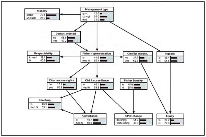
Source: Halls et al. (2002)
Halls et al. (2002) provide detailed guidelines for building models of co-management performance using GLMs and BNs which can be downloaded from http://www.fmsp.org.uk/r7834.htm. These are also included in Chapter 14 of Hoggarth et al. (2005). The guidelines include examples of models fitted to data compiled from co-management projects worldwide, as well as guidance on identifying sampling units, important variables, data levels and cleaning, exploratory analysis, sample sizes, and sensitivity analysis. More general guidance on GLMs can be found in McCullagh and Nelder (1989).
Table 6 provides a guide for selecting the most appropriate modelling approach based upon the expected response model and the number and type of variables to be included. Haddon (2001) provides useful guidance on fitting models to data illustrated with many spreadsheet examples.
TABLE 6
Guide to selecting appropriate empirical modelling approach (number of variables in parentheses)
| Response /performance variable | Explanatory variable | Response model | Appropriate method |
| Scale (1) | Scale (1) | Linear | Simple linear regression1 |
| Scale (1) | Scale (1) | Non-linear | Non-linear regression1 |
| Scale (1) | Scale (>1) | Linear | Multiple linear regression1 |
| Scale (1) | Scale (>1) | Non-linear | Non-linear regression1 |
| Scale (1) | Scale and Categorical (≥1) | Linear | General linear model |
| Categorical (≥1) | Scale and Categorical (≥1) | Linear or non-linear | Bayesian networks2 |
1 Other methods such as maximum likelihood may also be used.
2 Scale variables must first be grouped into class intervals.
3.5.3.1 Adapting and improving the plan
The empirical models of the type described above will evolve and their predictive capacity will improve through time as plans or strategies are adapted in response to the results of monitoring and evaluation activities. This cyclical passive form of adaptive management (see Box 10) may require several years of monitoring and evaluation at specific locations or waterbodies. There is also the risk that the best strategies will not be found because changes made to the plan may be too small to detect them. Evolutionary or trial-and-error adaptive management, where different strategies are tried more or less at random in the hope of accumulating experience about which one is best, may lead managers to eventually stumble upon the best strategy that may never have been identified on the basis of empirical models developed upon the basis of historical data. However, this form of adaptive management can be haphazard and wasteful (Hilborn & Walters 1992).
A number of alternative approaches are available to help managers evaluate and improve their management plans:
Each of these alternative approaches is briefly described below.
Refining and improving management plans and strategies on the basis of empirical models developed for specific locations or waterbodies could take years of formal monitoring.
| BOX 10 Passive adaptive management | |
| • | Monitors and evaluates the result of changes to the management plan or strategy |
| • | Compares the outcome with that in other places, or in previous times, and thus |
| • | Refines or adjusts the management plan based upon feedback and learning |
Appropriate administrative levels of government and intermediary organizations have the capacity to help accelerate this passive adaptive learning process by comparing management performance indicators and explanatory variables among sites, locations, fisheries or management units and feeding back lessons of success and failure to local managers or LMI via meetings, appropriate information networks, and media such as posters, radio transmissions, etc. (see Figure 4, Section 5.2.6). The prospect of enhanced learning capacity, achieved by sharing experiences may provide a strong incentive for LMIs to participate in more formal data collection programmes (see Section 5.2.5.5) that may also meet many of the needs of higher level managers (see Section 3.5.8).
Formal comparisons or the development of empirical models using the shared data (see below) and subsequent feedback may not even be necessary. Simply facilitating communication among LMIs by establishing, promoting and supporting appropriate communication networks or fora for sharing ideas and experiences may prove adequate without any formal comparisons (Section 5.2.6).
Because of the potential array of different management strategies and starting points that might be adopted at different sites or management units, this approach can overcome many of the problems associated with passive and evolutionary adaptive management adopted at specific locations or by individual fisheries (see Section 3.5.3.1).
| BOX 11 Learning lessons in Cambodia |
| “[In Cambodia] the CFDO expressed a great need for success and failure stories of community fisheries establishment and management…” (Felsing, 2004a). |
| BOX 12 Exchange visits in the United Republic of Tanzania |
| “[In Tanzania] village (exchange) visits have been regularly used as a way of raising awareness but also of bringing in new ideas to what may otherwise have remained a closed system. Representatives have been exposed to activities in neighbouring villages…and even to activities across the border in neighbouring Kenya” (Purvis, 2004). |
3.5.1.1 Quantitative comparisons and model development
Whilst the “among fishery or co-management unit comparisons” described above may be undertaken informally, for example, on a case study basis, it has long been recognized (Pollnac, 1994, 1998) that there are limits to what management can learn from qualitative case studies alone: “Numerous attempts have been made to summaries case studies…; nevertheless, decision makers are still faced with a bewildering array of allegedly crucial factors, with no way of evaluating their relative importance or interrelationships. It is clear that systematic, quantitative research is needed to provide a solution to this problem” (Pollnac, 1998).
Opportunities exist to develop quantitative empirical models of management performance from comparisons of case studies, fisheries or management units that can be used to guide management decision-making in respect of particular objectives. This kind of research could be undertaken by institutions such as fisheries departments, research institutes or other organizations with the necessary resources and institutional capacity.
Constructing empirical models of this type requires among fishery or co-management unit comparisons of a common set of quantitative indicators of both management performance and explanatory variables of the type described in Sections 3.5.1 and 3.5.2 above. Some variables such as catch and effort may have to be normalized by expressing them on a per unit area basis to make them comparable among sites. Other additional explanatory variables to those already contained in Table 3 may also need to be recorded to take account of natural environmental variation that is likely to exist among sites or locations. Examples might include the type of ecosystem exploited (river, lake, floodplain, etc.) or descriptors of the production potential of the site (e.g. % coral cover).
To illustrate the concept, suppose a number of local managers were interested in determining the number of “outsiders” they should allow access to their local resources (co-management units) without impacting on their own catches. By monitoring and comparing the total annual landings from their fisheries together with the total number of fishers participating (including outsiders), it may be possible to construct empirical models of the type illustrated in Figure 8.
FIGURE 8
CPUA vs. fisher density for 36 floodplain rivers in Africa ( ●); Asia ( ▲ ); and Latin America (■)
Source: Halls et al. (in press).
Curve is a least-squares fit to a modified Fox Production Model.
In this example, which is based upon a global comparison of floodplain fisheries, catches, measured in terms of catch per unit area (CPUA), can be seen to decline when total fisher densities exceed about 14 km-2. More local comparisons may generate different conclusions.
Multivariate models incorporating a range of different explanatory variables to predict other performance indicators can be constructed in a similar fashion using the General Linear Model (GLM) or Bayesian network (BN) modelling approaches described in Section 0).
This involves planned experimentation to identify optimal management strategies, for example optimal stocking densities for waterbodies with different rates of natural productivity. This experimentation approach requires greater organization and planning than the more passive or trial and error approaches, but the information gained should lead to better management and more consistent success. Further details of the approach and guidelines for implementation can be found in Garaway and Arthur (2002) and at the adaptive learning website http://www.adaptivelearning.info/.
Analytical models provide managers with a tool for predicting the effect of management interventions on the basis of established theories of fish population dynamics. They can be useful for answering questions such as: “What minimum mesh size would maximize yield from the fishery?” or “When would be the best month to close the fishery to maximize yield?” Constructing empirical models to answer these questions could take several years of monitoring and passive adaptive management.
In some cases, analytical models can provide answers to these types of questions using biological data sampled over relatively short periods of time. These biological data include fish length, weight, age, sex, and maturity and are used to estimate the population size or age structure, growth and mortality rates and spawning stock biomass as inputs to the models. Most analytical models provide advice only for fisheries that exploit single species. Therefore, they have limited utility for many co-managed fisheries that exploit multi-species assemblages with several gear types in a seasonal manner. For further guidance of analytical models and stock assessment and their data requirements see Hoggarth et al. (2005).
Medley (2004) describes a participatory approach to estimating levels of effort or catch quotas that maximize yield from a fishery. This Participatory Fisheries Stock Assessment (ParFish) method aims to improve the parameter estimates of production models of the type illustrated above by integrating the local ecological knowledge and experience of fishers into a Bayesian-based stock assessment. Local knowledge concerning catch rates, stock recovery time and stock size is elucidated using structured interview and questionnaire techniques. Prior knowledge of parameter values generated elsewhere or from earlier assessments can also be incorporated into the assessments along with model parameters estimated from depletion experiments and time series of catch and effort - effectively supporting an adaptive management approach. Further details of the methodology including guidelines and software are available at http://www.fmsp.org.uk/r8464.htm.
Analogous to the empirical modelling approach described above, local managers applying ParFish methodology might also mutually benefit from communication networks designed to support the sharing of knowledge, experiences and data among co-management units exploiting similar resources with similar technology. Sharing the results of depletion experiments, interview data and the outcome of previous assessments would promote a continually growing pool of common prior knowledge. Guidance notes for developing communication and information sharing networks is provided in Section 5.2.6 below.
The among fishery or co-management unit comparisons described in Section 3.5.4 also provides administrative levels of government with an opportunity to develop understanding of the effects of co-management policy on co-management performance (see Figure 4) and thereby also change policy in an adaptive manner.
By comparing important indicators of policy performance such as fish abundance (CPUE), food security, income, distribution of benefits, access to resources, conflicts, etc. (Section 3.2.2) against corresponding hypothesized explanatory variables monitored at or recorded for each co-management unit or fishery, it should be possible to draw conclusions about the effectiveness of existing policy either on a case-study basis or by building multivariate empirical models of policy performance using the General Linear Model (GLM) or Bayesian network (BN) modelling approaches described in Section 0. These models should also be able to provide insights into what changes to policy might be required to achieve desirable policy outcomes.
The selection of explanatory variables for inclusion in such comparisons or models of co-management policy can be guided by the Institutional Analysis and Design (IAD) Framework (Figure 9). Here, explanatory variables are described as “attributes” or “arrangements” that interact to produce outcomes or performance indicators. See Oakerson (1992) for a detailed explanation of the interactions. ICLARM (1998) and Pido et al. (1996) identify six main groups of attributes and arrangements (explanatory variables).
FIGURE 9
Institutional analysis and design framework
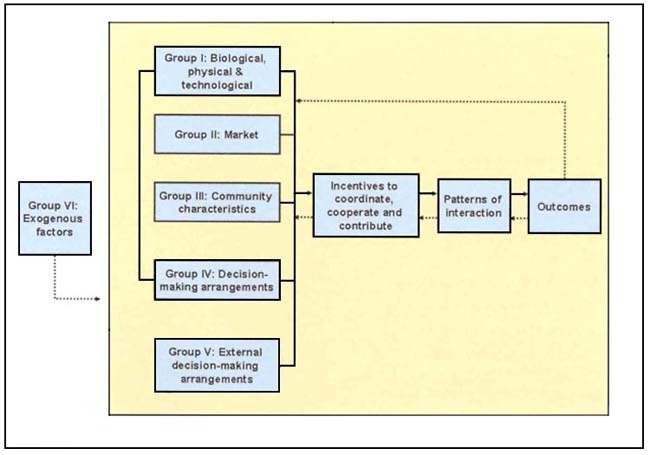
Source: ICLARM (1998)
Like the SL, the IAD framework is not a “cause and effect” model, but rather helps to logically structure information, identify and understand potential interactions and outcomes and test hypotheses. Managers may therefore find the framework useful for constructing a hypothesis matrix (see Table 7) to summaries hypotheses for testing or for summarizing explanatory variables selected for inclusion in multivariate models.
Since many of the explanatory variables should be recorded in the management plan (Section 3.3), negotiating a standard management plan format, should ensure that a common set of explanatory variables is available for comparison. A common set of policy performance indicators may also need to be negotiated with LMIs if participatory monitoring approaches are employed to provide the data (Section 5.2.5). Indeed, McArthur (1997) as cited by Estrella and Gaventa (1998) argues that the utility and cost-effectiveness of participatory monitoring approaches may be open to question unless site-specific research and innovations can provide the bases for planning and development at higher institutional levels. Alternatively, these indicators will have to be monitored under parallel monitoring programmes undertaken by the appropriate administrative levels of government (see Figure 4). Examples of indicators that might be selected for each explanatory variable group are given by Pido et al. (1996); Pollnac (1998); Preikshot and Pauly (1999); Berkes et al. (2001) and Ehler (2003). A selection of these is provided in Table 8.
TABLE 7
Hypothesis matrix summarizing potentially important explanatory variables in relation to co-management policy performance indicators. Ticks are only for illustrative purposes. Some may not be applicable, whilst other ticks may be appropriate.
| Co-management policy indicators | |||||||||
| Category | Example explanatory variables | CPUE1 | Food security | Income | Distribution of benefits | Poverty | Access to resources | Conflict | Compliance with rules & regulations |
| Group I: Biological, physical and technological attributes | Production potential | √ | √ | √ | √ | ||||
| Abundance/Biomass | √ | √ | √ | √ | √ | ||||
| Ecosystem type | √ | √ | √ | √ | |||||
| Water body type | √ | √ | √ | √ | |||||
| Rule enforcement potential | √ | √ | √ | ||||||
| Environmental health | √ | √ | √ | √ | |||||
| Habitat descriptors | √ | √ | √ | √ | |||||
| Exploitation intensity | √ | √ | √ | √ | √ | ||||
| Stocking density | √ | √ | √ | √ | |||||
| Habitat alteration activities | √ | √ | √ | √ | √ | ||||
| Group II: Market attributes | Economic value of resource | √ | √ | √ | |||||
| Market facilities/infrastructure | √ | √ | √ | ||||||
| Cost of marketing (market fees) | √ | √ | |||||||
| Price control mechanism | √ | √ | √ | ||||||
| Group III: Fisher community characteristics | Social cohesion | √ | √ | √ | |||||
| Dependence on fishery for livelihood | √ | √ | √ | √ | |||||
| Level of local (ecological) knowledge | √ | √ | |||||||
| Group IV: Decision-making arrangements | Legitimacy / widely accepted | √ | √ | √ | |||||
| Membership to decision-making body | √ | √ | √ | √ | |||||
| Clear access (property) rights | √ | √ | √ | √ | √ | ||||
| Management controls | √ | √ | √ | √ | √ | √ | √ | √ | |
| Representation in rule making | √ | √ | √ | √ | |||||
| Formal performance monitoring | √ | √ | |||||||
| Sanctions for non-compliance | √ | √ | √ | ||||||
| Group V: External decision-making arrangements | Enabling legislation for co-management | √ | √ | √ | |||||
| Local political/institutional support | √ | √ | |||||||
| Effective coordinating body | √ | ||||||||
| Group VI: Exogenous factors | External financial assistance | √ | √ | ||||||
| Capacity building support from NGOs | √ | √ | √ | ||||||
TABLE 8
Examples of explanatory variables and their indicators for comparing co-management policy performance indicators among co-management units, sites or locations.
| Category | Example explanatory variables | Example Indicators | Units | Notes |
| Group I: Biological, physical and technological attributes | Production potential | Water transparency (Secchi depth) | m | May not be valid indicator in rivers |
| Primary production | 0;1;2 | g/C/m/2 year: Low <150 (0); medium 150–300 (1); high >300 (2) | ||
| Abundance/Biomass | Annual catch per fisher | Tonnes/fisher | All species combined or specify for each target species. | |
| Ecosystem Type | Ecosystem Type | 0;1;2..n | River (0); fringing floodplain (1); beel (2); lake (3) | |
| Water body type | Permanence | 0;1;2 | Seasonal (0); perennial (1); both (2) | |
| Rule enforcement potential | Area under co-management per fisher | km2/fisher | or km of coastline/fisher (specify) | |
| Environmental health | Health of critical habitat | 0;1;2 | Low (0); medium (1); high (2) | |
| Nutrient recycling | Depth of reserve, lake, fishing area | m | ||
| Habitat descriptors | % Coral cover | % | ||
| Exploitation intensity | Fisher density | N / km2 | or km of coastline (specify) | |
| Number of villages | N | |||
| Mean size of fish caught in month x, with gear x | cm | |||
| Stocking density | Stocking density | kg/ha | ||
| Habitat alteration activities | Habitat alteration activities | 0 i– 5 | Destructive (0); none (1)……beneficial (5) | |
| Group II: Market attributes | Economic value of resource | Mean unit value of target species | US$/kg | |
| Market facilities/infrastructure | Transport/infrastructure/landing sites | 0;1;2 | Poor (0); medium (1); good (2) | |
| Cost of marketing (market fees) | Cost of marketing (market fees) | 0;1;2;3 | None (0); low (1); medium (2); high (3) | |
| Price control mechanism | Price control mechanism | 0;1 | No (0); yes (1) | |
| Group III: Fisher community characteristics | Social cohesion | Social cohesion | 0;1;2 | Low (0); medium (1); high (2) |
| Dependence on fishery for livelihood | % of household income derived from fishing | % | ||
| Level of local (ecological) knowledge | Level of local (ecological) knowledge of fishers | 0;1;2 | Low (0); medium (1); high(2) | |
| Group IV: Decision-making arrangements | Legitimacy / widely accepted | Legitimacy of local decision-making body | 0;1;2 | Low (0); medium (1); high (2) |
| Membership to decision-making body | Democratically elected | 0;1 | No (0); yes (1) | |
| Clear access (property) rights | Clear access (property) rights | 0;1 | No (0); yes (1) | |
| Management plan | Present/carried out | 0;1 | No (0); yes (1) | |
| Management controls | Mesh/gear size restrictions | 0;1 | No (0); yes (1) | |
| Gear ban(s) | 0;1 | No (0); yes (1) | ||
| Closed seasons | 0;1 | No (0); yes (1) if yes specify month(s) closed | ||
| Reserve area as a % of total management area | % | |||
| Representation in rule making | Representation in rule making (fishers) | 0;1;2 | Low (0); medium (1); high (2) | |
| Formal performance monitoring | Formal performance monitoring by community | 0;1 | No (0); yes (1) | |
| Sanctions for non-compliance | Sanctions for non-compliance | 0;1 | No (0); yes (1) | |
| Group V: External decision-making arrangements | Enabling legislation for co-management | Enabling legislation for co-management | 0;1 | No (0); yes (1) |
| Local political/institutional support | Local political/institutional support | 0;1;2;3 | Anti (0); Weak (1); indifferent (2); strong (3) | |
| Effective coordinating body | Nested structure | 0;1 | Absent (0); Present (1) | |
| Group VI: Exogenous factors | External financial assistance | Expenditure on community | $/year/fisher | |
| Capacity building support from NGOs | Support for community from NGO's | 0;1;2;3 | none (0); weak (1); medium (2); strong (3) |
6 See discussion on hyper-depletion and hyper-stability in Hilborn and Walters (1992).
![]()
![]()
![]()