The purpose in the discussion which follows is to establish a sound basis, both in terms of genetic theory and in the light of experimental evidence, for a rational choice of breeding or crossbreeding strategy in any particular case.
First, however, it is useful to set crossbreeding options in context with selection alternatives. Selection within populations is based on a simple additive model of gene action. In practice it generally delivers genetic gains in line with theoretical expectations (Smith, 1984).
Crossbreeding is often regarded as an alternative to selection. It therefore needs to be stressed that these are not mutually exclusive strategies, and that any of the crossbreeding options discussed here requires a supporting selection program, either in the contributing pure breeds, or in the resulting synthetic. The relationship between possible selection and crossbreeding strategies in a typical local dairy cattle population where crossing with an exotic breed is being contemplated is illustrated in Figure 2.1
The average performance of a group of animals is determined by their genetic capacity and by the environmental conditions in which they are kept. Sometimes the genetic and environmental components interact, e.g., when genetic differences between animals are larger in one environment than in another.
The genetic component is the aggregate effect of the actions of innumerable genes acting individually and in concert with other genes or groups of genes in the System. The bovine genotype has of the order of three million such genes. Many are no doubt functionless as far as any particular trait is concerned. Much is known about the biochemical structure and function of some genes. For most, however, we have no such information. Since there is little evidence that individual genes have major effects on most economic traits, it would in any case be difficult to use such information for the purposes of genetic improvement.
The genetic models from which we develop working procedures for breeding programs therefore begin at the level of the gene. Since gees occur in pairs, and are also grouped in chromosomes, it is convenient to consider gene effects at three levels:
- Additive effects: the effects due to single genes acting independently of the remainder of the genotype.
- Dominance effects: the effects due to the joint action of gene pairs within loci.
- Epistatic effects: the effects due to the joint action of two or more genes at two or more loci.
Selection theory is based on the accumulation of favourable additive effects from generation to generation. Crossbreeding theory is largely (though not exclusively) based on the arrangement of favourable dominance effects in each generation. These dominance effects are not cumulative from one generation to the next, though they can be enhanced by appropriate selection (e.g., Rich and Bell, 1980; Orozco, 1976). Epistatic effects can take an infinitenumber of forms involving any number of genes and any number of loci. It is therefore impossible to build any general consideration of epistatic effects into either selection or crossbreeding models.
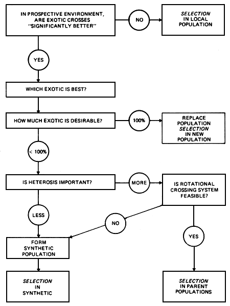
Figure 2.1 Strategic options involving crossbreeding and selection.
In the discussion which follows, the main emphasis is on the development of models for crossbreeding based solely on additive and dominance effects. In many cases, these are a fully adequate basis for breeding decisions.
The main factors which can render these models inadequate in certain cases are (1) the presence of epistatic effects (2) the presence of maternal effects (3) interaction of genotypic effects with environmental factors. These factors are discussed separately.
This is the name used for a model which includes only additive and dominance effects. In the case of an individual (or group) produced by combining two separate genetic strains through some crossing System, the additive component is proportional to the gene contribution from each strain. For example, in a first cross (F1) between two strains (P1 and P2) the additive value is 1/2 (P1 + P2). The additive value of a backcross to strain 1 (B1= P1 × F1) is 3/4 P1, + 1/4 P2.
The dominance value is somewhat more complex. Since it is made up of the aggregate of dominance effects at many separate loci, it can be explained best by considering it first at one locus. Assume that for any particular locus, there are two alleles, A1 and A2 with frequencies p and q. Define the present genotypic mean, determined by ail other loci except this one, as μ. Let the value of the genotype A1 A2 then be μ + a, that of the genotype A2 A2 be μ - a and that of the heterozygous genotype A1 A2 be μ + d. This situation is illustrated in Figure 2.2 for four different degrees of the dominance effect, d.
It is clear that d is simply the deviation of the heterozygote A1 A2 from the average of the two homozygotes A1 A1 and A2 A2. For reasons which are discussed below, it has generally been found that these dominance effects are positive. The mean genotype is then the average of the three genotypic values, which is obtained by multiplying each of them by its frequency and summing these products:
Mean = p2(μ + a) + 2pq(μ + d) + q2(μ - a)
= μ + (p - q) a + 2pqd
In the absence of selection, efforts to increase or decrease the level of heterozygosity in a population do not of themselves change gene frequencies - they merely change the relative proportions of homozygotes and heterozygotes. The first two terms in this equation are therefore not affected by increasing or decreasing heterozygosity. The third term is simply the product of the frequency of heterozygotes and the dominance effect at that locus. Given that there is some dominance, the mean genotypic value is then a linear function of the proportion of heterozygotes.
This model relates to a single locus. Extended to N independent loci, it says that the mean genotypic value in the population is a linear function of the average heterozygosity at ail loci at which some dominance exists. The nature of the dominance effect does not need to be specified - there may be partial, complete or overdominance at any or ail of these loci.
Fisher (1931) developed the argument that evolution will tend to have produced dominance of favourable genes, and recessiveness of deleterious genes. He suggested that this is brought about by the effect of selection acting on genes (at other loci) which modify the value of the heterozygote. Wright (1977) and Kacser and Bums (1981) have shown that the evolution of dominance is more likely to be a consequence of the way enzymes interact in metabolic pathways. Most experimental evidence confirms that disadvantageous mutants tend to be recessive. The widespread occurence of dominance (partial, complete or over-dominance) of favourable alleles provides the basis for the general expectation that at any particular locus the heterozygote will be better than the mean of the two corresponding homozygotes. Carried through to N loci, this leads in turn to the expectation that the mean genotypic value of the population should increase linearly as heterozygosity increases.
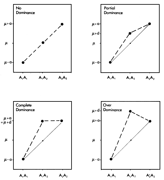
Figure 2.2 Different degrees of single locus dominance.
The sum of ail positive or beneficial dominance effects at individual loci is the basis of the broader concept of heterosis. Heterosis is defined as the deviation (positive or negative) of an individual or group from the mean of its parents. Because heterosis is almost exclusively the aggregate of ail single locus dominance effects, and because these are usually positive or beneficial, heterosis can be expected also to be usually in a favourable direction. This has generally been found to be the case.
Arising from the single locus model, the heterosis effect is also expected to be a linear function of the level of heterozygosity. Extending the Additive-Dominance model from its single-locus version to the level of a multi-locus trait, we can say that the expected average performance of any group of individuals produced by combining the genetic resources of two parental strains through some form of crossbreeding will be
μ + X1 A + X2 H
In this model, is the overall mean value in the population, A is the additive difference between the two parental strains, and H is the heterosis displayed by their F1 offspring. Note that A is the sum of the additive gene effects for which the parental strains differ, and H is the sum of the dominance effects created when the two strains are crossed. The weighting factor X1, measures the proportion of genes contributed by the two strains, and X2 measures the level of heterozygosity. If the additive difference A is defined as P2 - P1, then μ can arbitrarily be set equal to P1 and X1 will simply be the proportion of genes contributed by the second parent, P2. From the mating System that is used to produce any particular crossbred group, the value of X2, the expected heterozygosity level, can readily be calculated.
In order to predict the genetic value of a crossbred group therefore, we need to know four quantities: A, H, X1 and X2. The two weighting factors X1 and X2 can be deduced from the mating or breeding structure. The values of A and H need to be estimated from actual data. The real purpose of experiments intended to clarify crossbreeding options is therefore the estimation of A and H.
The use of this model to describe or predict the genetic value of a group can be illustrated by applying it to the first four types of crossbreds which can be produced from two parental breeds or strains. These types or groups are
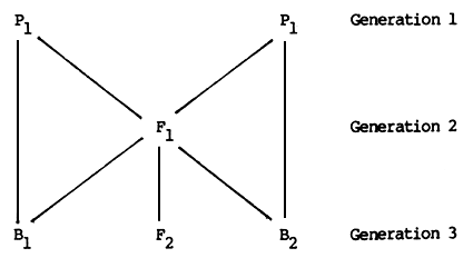
P1 and P2 are the parental strains, e.g., Sahiwal and Holstein breeds. F1 is the first crossbred generation, produced by mating Sahiwal cows to Holstein bulls (or vice versa). F2 is the second crossbred generation, produced by mating F1 bulls to F1 cows. B1 and B2 are backcrosses to Sahiwal (P1) and Holstein (P2) respectively, produced most conveniently by mating Sahiwal and Holstein bulls to F1 females. In each case, the reciprocal crosses (i.e., F1 bulls mated to Sahiwal and Holstein cows) could also be used to produce the same génotypes.
The difference between the parental breeds is P2 - P1= A. The heterosis shown by the F1 is F1 - (P1 - P2)/2 = H. The expected value of each group is then as follows.
P1 = μ
P2 = μ + (1)A
F1 = μ + (1/2)A + (1)H
F2 = μ + (1/2)A + (1/2)H
B1 = μ + (1/4)A + (1/2)H
B2 = μ + (3/4)A + (1/2)H
The relationships between these six genetic groups are illustrated in Figure 2.3.
Since the expected performance of each group is a function of two factors, A and H, it can be displayed by superimposing the heterosis effect H on the additive effect A. The result is a diagram which has some resemblance to the front elevation of a classical Greek temple, and is therefore called the Greek Temple Model (Cunningham, 1987).
It is clear that, provided this Additive-Dominance model is appropriate, the expected value of any group resulting from a crossbreeding scheme can be predicted if we know the values of A + H and can state (i) the proportion of genes from the two parental strains and (ii) the proportion of maximum heterozygosity. In the following section, a number of crossbreeding Systems are considered using the framework provided by this model.
A synthetic population can be formed by inter se mating from any crossbred group. The simplest form of synthetic, with two parental breeds, is formed from the F1 generation. The performance of the F2 and subsequent generations can be readily predicted. On average, they contain a 50% gene contribution from each parental breed, and therefore have half of the additive effect. They also, on average, retain 50% of the heterozygosity of the F, generation, and therefore should display half of the heterosis effect.
Synthetics may also be formed from any other crossbred group, for example, a backcross to the superior breed. This will have three-quarters of the additive effect, and should have 37.5% of the heterosis effect. In general, the proportion of maximum heterozygosity, and hence of heterosis, retained in synthetic populations is (Dickerson, 1973)

where P1 is the proportion of genes contributed to the synthetic by the ith source breed. Thus, a synthetic started from a backcross will have .75 of its genes from one breed and .25 from the other. The proportion of heterozygosity retained is then
1 - .752 - .252 = .375
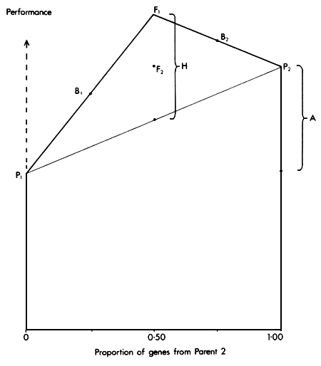
Figure 2.3 The Greek Temple Model, showing the expected performance of parental (P1 and P2), F1, F2 and backcross (B1 and B2) groups as functions of Additive (A) and Heterosis (H) effects.
In the context of crossbreeding between Bos taurus and Bos indicus, we are usually dealing with two breeds only - one from each type. Where a third breed is involved it is usually a second Bos taurus type. Heterosis between Bos taurus breeds is usually very low by comparison with that found for taurus-indicus crosses. In considering such three breed synthetics therefore we are usually concerned only to measure how much of this taurus-indicus heterosis is retained. This can be calculated simply by considering the two Bos taurus contributing breeds as if they were one.
The proportion of heterosis retained in synthetics formed with various proportions of Bos taurus and Bos indicus is then as follows:
| PROPORTION OF GENES FROM | PROPORTION OF HETERDSIS RETAINED IN SYNTHETIC | |
| TAURUS | INDICUS | |
| .125 | .875 | .22 |
| .25 | .75 | .375 |
| .375 | .625 | .47 |
| .5 | .5 | .5 |
| .625 | .375 | .47 |
| .75 | .25 | .375 |
| .875 | .125 | .22 |
Since a synthetic can be formed by inter se mating of individuals with any level of gene proportions from the two parental breeds, the expected performance of synthetics then forms a continuous curve on the Greek Temple diagram (Figure 2.4). For any given gene proportion, the synthetic is always inferior to the original cross from which it was formed.
A rotational cross between two breeds is established by using pure bred males of each breed in alternate generations. The first generation is clearly an F1, but after a few generations the population has a two-third gene complement from one parental breed, and one-third from the other. In each following generation, the two parental breeds still contribute two-third and one-third of the gene complement, but the position of the two breeds is reversed. In each generation, the breed contributing two-thirds of the gene complement is the breed which most recently provided the males to the mating system.
In each generation, the proportion of maximum heterozygosity retained is two-thirds, and therefore the expected performance includes two-thirds of the heterosis effect.
The performance of animals in two successive generations of a two breed rotation is thus
μ + 1/3A + 2/3H and
μ + 2/3A + 2/3H.
If A is large, then these two generations may differ substantially in performance. With overlapping generations, the population would then contain animals of quite variable type and production levels, and this can be a serious disadvantage.
Figure 2.4 shows the two positions occupied by alternate generations of a two breed rotation relative to the parental breeds, F1, backcrosses and synthetics.
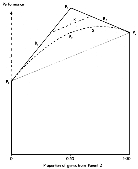
Figure 2.4 The Greek Temple Model, showing the expected performance in Rotational (R) and Synthetic (S) breeding systems
The previous discussions have ail been based entirely on the additive-dominance model. The following are the three main factors which can, in some circumstances, render this model inadequate.
Epistatic effects. The term epistasis is used to describe ail multiple gene effects which involve more than one locus. The simplest such effect is the joint effect of two genes at two separate loci. This specific kind of epistatic effect is an additive by additive effect. The joint effect of a single gene at one locus and a gene pair at a second locus is another form of epistasis, called an additive by dominance effect. If we limit consideration to two loci, there are possible four such additive by additive effects, four additive by dominance effects and one dominance by dominance effect, or a total of nine specific types of epistatic effect. These may be positive or negative. Cockerham (1954) has written a general model to accommodate these effects. It is, however, difficult to measure the effects in practice.
Using differing specifications of the effects, Dickerson (1973), Kinghorn (1980), Hill (1982) and Sheridan (1981) have given the expected performance of different types of crosses, taking account of two locus epistasis. Koch et al (1985) discuss the relationships between the first three of these formulations of epistasis. In ail cases, the loss of beneficial epistatic effects in F2 and backcross generations, and in rotational and synthetic populations led to the expectation of lower performance in these cases than would be predicted solely from the additive-dominance model.
If consideration is extended to three or more loci, then the number and kind of possible epistatic effects increases rapidly, and genetic models are of purely theoretical interest. Attempts to interpret deviations from the additive-dominance model in terms of epistasis have therefore largely been limited to consideration of two locus epistasis.
What evidence is there of the existence of significant epistatic effects? Cunningham (1982) concluded that the great majority of analyses reported in mice, dogs, corn and beef cattle supported the adequacy of the additive-dominance model. Sheridan (1981) presented evidence in poultry, showing that this model was insufficient. In particular, his data showed performance in the F2 substantially below expectation. The data from Bos taurus - Bos indicus crossbreeding trials, summarised by Syrstad (See Section 5.7), suggest that a similar situation may obtain for first lactation milk production, though for other traits the additive-dominance model seems adequate.
In the context of planning dairy cattle crossbreeding in the tropics, therefore, it seems reasonable at the present state of knowledge to develop the plans using the additive-dominance model. However, a particular aim of future crossbreeding experiments should be to further test the validity of this model.
Maternal effects. Some traits are substantially effected by the maternal environment. This is particularly the case where the offspring are reared on the dam, as in most sheep, beef cattle and pig production Systems. In such cases, the maternal, effect, like other effects with a genetic component, can have both additive and dominance components. Under the same assumptions as before, these lead to additive and heterosis effects which are proportional to the gene complement in the dam, and to the fraction of maximum heterozygosity in the dam. Where necessary, these elements can be added to the model, and can be estimated from appropriate analyses. The models are discussed in Dickerson (1973) and a good example involving beef cattle is given by Koch et.al.(1985).
In the context of dairy cattle crossbreeding in the tropics, maternal effects can generally be ignored. The reasons for this are first that the calves are generally reared artificially from birth, and secondly that the traits of most interest are recorded after a long interval of separation between dam and offspring. Maternal effects are therefore not taken into account in the models elaborated here.
Genotype by environment interaction. Both additive and heterosis effects can vary with environmental level. Additive by environment interactions are well documented. There is less evidence for interaction of heterosis by environment interaction. However, the review by Barlow (1981) concluded that it was more often the rule than the exception.
These interactions are of obvious importance in predicting the consequences of different crossbreeding Systems. Since the predictions in all cases depend on the estimated level of additive and heterosis effects, the accuracy of the predictions depends on the validity of these estimates in the environment in which the crossbreeding system is implemented. The existence of interactions will also mean that the crossbreeding Systems appropriate, with a particular pair of breeds, in one location may not be appropriate in another environmental situation.
Figure 2.5 illustrates a range of situations in which the absolute and relative sizes of the additive and heterosis effects vary. Three levels of the additive effect are included (A = 80%, 40% and 20% of mid-parent value). Likewise, three levels of heterosis effect are used (H = 40%, 20% and 10% of mid-parent value). It can be seen, by reference to Figure 2.4, that the expected performance levels of the parents, F1, F2_, backcrosses, rotation and synthetic groups relative to each other will ail depend on the absolute and relative levels of both A and H. These in turn may, for a given pair of breeds, depend on the environment.
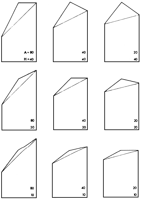
Figure 2.5 Greek Temple Models illustrating nine combinations of levels of A (80, 40 and 20%) and H (40, 20 and 10%)