![]()
![]()
![]()
1. Inventories
2. Estimating forest resources
3. Growth and productivity
4. Some data on productivity
5. Allowable cut and compartment layouts
6. The main technical approaches
7. Measurement of fodder biomass and density of cover
8. Evaluation and monitoring of resources: the new tools
This chapter summarizes the main methods for observing and measuring the arboreal, woody and herbaceous components of the forest ecosystems in dry tropical zones. At the end of this chapter, the methods for evaluating and monitoring the resources are described.
1.1 Regional or global inventories
1.2 National inventories
1.3 Local inventories
Inventories should provide quantitative and qualitative evaluations of the resources and their distribution with the necessary degree of accuracy according to the particular objectives to be attained. Because of the wide variety of different objectives, inventories exist for large geographic regions, and even whole continents, countries, administrative sub-regions and forests. These have been established for macroeconomic, bio-geographic, physical planning purposes, as aids for local management purposes. Each one of these has specific, if not unique, methods of observation and evaluation techniques. This is due to the diversity of the situations, but becomes more controversial when this diversity is due to a lack of minimum standardization or communication. It is therefore an area which demands a major effort to standardize practices and gather information. We would add that this could be encouraged by improving certain monitoring and observation techniques (using radar satellite imagery).
A distinction is normally drawn between three major types of inventories: regional or global, national and local. For the forest manager the latter two are the most relevant. National inventories are associated with physical planning, and local inventories with forest management.
These are based on macroeconomic or bio-geographic approaches and only provide quantitative or qualitative global evaluations relating to the fauna, flora and sometimes the elements examined for a mesological approach. These mainly refer to forests in the strict sense of the term, ignoring small rural wood-lots, agroforestry cover and in particular woody plants scattered around fields constituting a substantial biomass. The latest global and regional inventory was the one drawn up by FAO (1993) which excluded the densely cultivated zones from the dry regions.
This is the most common tool used for physical planning and national forest management. It is a national planning tool. It is clearly more detailed than the regional inventories just mentioned, because it describes, quantifies and identifies the site of the resources more precisely, but in particular it relates the forest to other agricultural, urban and industrial components in the territory. It should therefore take account of the ‘off-forest’ woody resources, but this is not always done.
Emphasis on the importance of the off-forest resources is based on an estimate by Jensen (1995) regarding the volume of wood taken from the fields, namely, that at the national level, the growing trees on fallow land and crops account for 30 percent of the wood resources in Burkina Faso and 19 percent in the Gambia (Box 10 and Table 6).
For the same reasons, it should be noted that the total output (namely wood, fodder and farm production) of a forest-park or shrub-fallow land may exceed the total output of a forest. In some parks, the trees are better protected against fire, and the density of the shoots is not so great which gives them greater individual growth; in a forest stand, competition from the grass cover from the time of the first rains reduces water availability and hence limits growth. Strictly from the wood production point of view, the disappearance of the forests to the benefit of the parks carrying trees for multiple uses is not always disastrous. In future, in the dry tropical zones, cultivated lands will certainly be increasingly used for wood and fodder production, and can be incorporated into the national inventory.
National inventories have been drawn up in many countries, particularly in West Africa: Burkina Faso (Table 6), the Gambia (Box 10), and Senegal (Box 11). Mali decided on an inventory of the southern part of the country, and this was completed in 1991 (Table 7). Niger has a regional inventory dating back to 1986, and the Planning and Utilization of Soil and Forest (Planification et Utilization des Sols et Forêts) project worked from 1984-1989 on the inventory of wood tree sources in the non-desert part of the country. This inventory was updated (Landsat TM [thematic mapper]) by the Energy II project (Energie II).
For the developing countries, the methodological difficulty is transferring the results of the national inventories in order to provide data that can be used for local development and planning. This is an avenue of research to be undertaken in future, because there is so much pressure that these wood stands are rapidly being changed by the local people. It is therefore vitally important to begin sustainable sub-management of all the forest stands in every country, as Niger is doing (SEED-CTFT, 1991), using all available inventories.
| Box 10: National forest inventory in the Gambia The Gambia has a national inventory since 1980 (Forester, 1983). The mapping of stand types was implemented through interpretation of a complete set of panoramic, panchromatic and infra-red photographs at scale 1/25 000 dated October 1980. The background map is a mosaic of panchromatic photographs enlarged to scale 1/10 000. The volume is measured over bark, starting from a 5 cm above ground felling point. It concerns all trees whose diameter at 1.30 m is superior to 10 cm. Trees under 10 cm diameter are numbered and accounted for as regeneration. The inventory covered almost the entire territory, including trees on cropland. Some 590 inventory plots out of 2 035 were established on non-forested village land. Several volume tables were used for timber as well as for fuelwood species. For trees under 40 cm diameter, the volume tables for timber species correspond to those established for fuelwood species. For large dimensions (over 60 cm diameter), timber volume tables are 7.5 percent superior to fuelwood volume tables. Growth increments have not been measured. They were estimated using sophisticated mathematical applications based on hypothesis which were not verified. Distribution of surface areas, volumes, wood productivity and regeneration
under various natural vegetation formations in the Gambia (DFS/GTZ, 1983). |
||||||
| Type vegetation formations |
Area |
Volume |
Increments |
Regeneration |
||
| 1000 m3 |
(m3/ha) |
(1000 m3/year) |
(m3/ha/year) |
(number/ha) |
||
| Mangrove |
14 980 |
2 748 |
183.5 |
72 |
4.8 |
609 |
| Woodland and woodland savanna |
89 446 |
5 217 |
58.3 |
123 |
1.4 |
860 |
| Shrub savanna |
346 981 |
5 370 |
15.5 |
156 |
0.4 |
1 075 |
| Total forest formations |
451 407 |
13 335 |
29.5 |
351 |
0.8 |
1 016 |
| Fallow and cropland |
394 423 |
3 213 |
8.1 |
56 |
0.14 |
847 |
| Total natural formations inventoried |
845 830 |
16 548 |
- |
407 |
- |
937 |
| Source: Jensen, 1995 |
||||||
| Vegetation formation types |
Area (1000 ha) |
Volume in (1000 m3) |
Volume (m3/ha) |
Increments |
|
| (1000 m3/year) |
(m3
/ha/year) |
||||
| Woodland and woodland savanna |
4 848 |
193 803 |
40.0 |
- |
- |
| Shrub savanna and ‘tiger’
thickets |
10 572 |
155 545 |
14.7 |
- |
- |
| Total and average for forest formations |
15 420 |
349 348 |
22.7 |
8 595 |
0.56 |
| Fallow and cropland |
8 770 |
152 851 |
17.4 |
1 684 |
0.19 |
| Total inventoried and average |
24 190 |
502 199 |
20.8 |
10 279 |
0.42 |
| Box 11: National forest inventory in Senegal Senegal has a national inventory that was drawn up in 1978. The cartography of the different types of forest stands was based on Landsat MSS (multi-spectral scanner) image interpretation on a scale of 1:500 000 in 1978, whose pixels represented an area 57 × 79 m (0.45 ha). The cartography only covered forest stands. The volume inventory was never made but the average volumes of different types of stands has been estimated on the basis of data from different inventories and measurements made by the Forestry Service (Service Forestier) and the National Forestry Research Centre (Centre National de Recherches Forestières). It indicates the volume of greenery on bole overbark to the 7 cm cut of all trees with a diameter above 10 cm. The range begins at 0.25 m3/ha for the shrub steppe to 120 m3/ha for the closed forests. In order to express the total volume (trunk + branches up to 4 cm in diameter) the bole volume must be multiplied by 1.4. To estimate productivity, the figures used range from 0.02 m3/ha/year
for the shrub steppes to 3 m3/ha/year for the closed forests.
These estimates are multiplied by the area of the stand types taken from
the cartography. |
|||||
| Forest areas, bole
volume and fuelwood productivity of different types of stands in the 1978
Senegal National Forest Inventory |
|||||
| Wood stands |
Area 1978 |
Volume |
Increments |
||
| 1000 m3 |
m3/ha/year |
1000 m3 |
m3/ha/year |
||
| Mangrove |
169 |
5 936 |
35.1 |
- |
- |
| Closed forest |
13 |
4 500 |
104.5 |
26 |
2.0 |
| Galery forest |
45 |
1 560 |
104.5 |
135 |
3.0 |
| Open woodland |
349 |
20 952 |
60 |
699 |
2 |
| Savanna woodland |
2 500 |
73 557 |
29.4 |
3 702 |
1.5 |
| Tree savanna |
4 852 |
28 209 |
5.8 |
3 229 |
0.7 |
| Shrub savanna |
469 |
432 |
0.9 |
64 |
0.1 |
| Tree steppe |
46 |
455 |
9.9 |
23 |
0.5 |
| Tree steppe and grassland |
3 159 |
3 248 |
1 |
367 |
0.1 |
| Tree and shrub steppe |
2 160 |
326 |
0.2 |
52 |
0.02 |
| Palm groves |
40 |
- |
- |
- |
- |
| Coastal thicket |
43 |
- |
- |
- |
- |
| TOTAL |
13 845 |
139 175 |
- |
8 297 |
- |
|
NB: The rural woodlands are not included in this estimate. Source: CTFT/SCET, 1981 |
|||||
| Vegetation formations |
Rainfall |
Gross volume |
Dominant height |
Dominant species |
| Open woodland with Isoberlina doka |
935-1 085 |
39-61 |
13-15 |
Isoberlina doka |
| 1 295-1 355 |
34-90 |
11-14.5 |
Isoberlina doka |
|
| Other open woodlands |
1 000-1 310 |
50-58 |
11.1-11.8 |
Daniellia oliveri |
| Shrub savanna (sand dominant) |
500-700 |
4.5-10.1 |
4.9-7.9 |
Guiera senegalensis |
| Hard pan plain-land stands |
450 |
5.5-6.0 |
5.5-9.4 |
Pterocarpus lucens |
| Shrub savanna (heavy soils) |
450-575 |
2.7-8.7 |
4.3-8.3 |
A. seyal, Balanites aegyptiaca |
| South Sudanian shrub savanna |
980 |
15.4-18.9 |
6.4-7.3 |
Terminalia macroptera etc. |
| Tree savanna (hydromorphic soils) |
630-700 |
7.7-16.2 |
7.4-10.3 |
A. seyal, A. leiocarpus, etc. |
| Tree savanna (non-hydromorphic soils) |
560-700 |
10.5-18.4 |
8.3-11.5 |
Combretum spp., etc. |
| South Sudanian savanna |
935-1 085 |
25.0-57.6 |
8.8-11.7 |
Pterocarpus erinaceus |
| Sudano-Guinean tree savanna |
- |
22.0-45.7 |
8.7-11.3 |
D. oliveri, P. erinaceus |
| A few South Sudanian and Guineo-Sudano
‘orchards’ |
975-1 310 |
21.3-27.4 |
8.3-10.5 |
Vitellaria paradoxa |
NB: The gross volumes and dominant heights are the extreme per type of stand. For each type of stand several sites were inventoried and their averages recorded.Source: Nasi and Sabatier, 1988a
a) General features
Local inventories relate to forests for which management actions are intended. In order to define the objectives and the management procedures correctly, it is essential for a prior survey of the human and physical environments interacting with the forest to be carried out, and in particular to specify the socio-economic and environmental roles of these environments. This will partly facilitate the definition of the variables (to be measured and/or benchmarked). They also make it possible to spell out more clearly such more general and global aspirations as the notion of sustainability. This situation must then be coupled with a geographical description and demarcation of the forest and the zones which are only slightly forested, agriculture and rural.
Before drawing up the inventory, the forest may also be divided up into to several complementary partitions. In particular, zoning can be carried out in terms of usage, and in terms of the major vegetation stands. Photo-interpretation and remote sensing are valuable tools for the latter, the first being based upon surveys or field observation. Lastly, the forest manager must also have a stratification so that the inventory can be adapted to each layer. After this, the techniques used will be taken from the traditional methods that are always used when carrying out stratified surveys.
Whether a priori stratification is used, which is the method advised, or whether this is done a posteriori, as is often necessary because of time and cash constraints, in most cases the survey is carried out systematically in the areas identified, set out regularly along equidistant rows. A preliminary sample with a very low rate should be envisaged in order to characterize the heterogeneity of the resources, namely the value of the variation coefficients of the variables studied, in order to be able to estimate the minimum number of experimental plots necessary to achieve a specific level of precision.
| Box 12: Sample size Let us take a population P of N individuals and a variable X which for individual i has the value Xi. The average 0 of N values Xi may be estimated as the average of the Xi measured on a sample of size n. Using the traditional hypotheses: sample without remainder, random and Gauss distribution of X (the normal law), one can construct a confidence interval of 0 at level 95 percent which is written as follows: Noting the precision (CV is estimated by
NB: N is the number of potential plots in the area inventoried;
n is the number of plots measured. X may be a volume, a land area, a height...
attached to each plot. |
The size of the experimental plots being surveyed generally varies between 0.1 and 0.5 ha. It would appear that an area of 0.125 ha (25 × 50 m for example) is a good compromise between the desire to reduce the percentage of error and to economize on time and money.
On the basis of a study carried out in the Koumpentoum Forest in Senegal, Arbonnier (1990) estimated that a 1 percent survey rate, representing the ratio between the total area sampled and the total area of the forest, is acceptable for making a partition of the forest into homogeneous compartments each of 500 ha for a silvo-pastoral management scheme (Figure 6). He also showed that accuracy has nothing to do with the shape or the size of the experimental plots (Box 13).
Table 8: Values of several coefficients of variation (inventoried) in the literature
| Forest-Country |
Vegetation |
Rainfall (mm) |
Experimental plots |
CV % |
References |
| Woro-Mali |
Shrub and tree savanna |
600-700 |
0.1 ha |
CV(N) = 68.9 |
Parkan |
| Yabo-Burkina Faso |
Riparian formation |
600 |
0.25 ha |
CV(Vol) = 79.8 |
Compare |
| Dabo-Senegal |
Open woodland and |
800-1 000 |
0.5 ha |
CV(N) = 31.5 |
Fall, Gueye 1993 - a and b |
| Faira-Niger |
Striped and leopard bush |
600 |
0.1 ha |
|
|
| 2 < diameter < 8 cm |
|
|
CV(Vol) = 35-60 |
Mengin-Lecreulx |
|
| 8 < diameter < 20 cm |
|
|
CV(Vol) = 65-85 |
Chabanaud, 1986 |
|
| Diameter > 20 cm |
|
|
CV(N) = 100 |
|
|
| Faya-Mali mountains |
Poor to rich formation |
750-1 000 |
0.2 ha |
CV(G) = 37 |
Sabatier, Nasi, 1988 |
| Morondava-Madagascar |
Dry closed forest |
500-1 000 |
Sample strip 40 ×
1 000 |
|
|
| Species harvested |
|
|
CV(Vol) = 28 |
|
|
| Species harvested |
|
|
CV(N) = 33 |
|
|
| Not harvested species |
|
|
CV(N) = 49 |
|
CV = Coefficient of variationFigure 6: Partition of the forest into homogeneous compartments each of 500 ha for a silvo-pastoral management scheme
Vol = Volume/ha
N = Individuals/ha
G = Basal area/ha
Stem: diameters measured at collar height < 20 cm
Foot: diameters measured at collar level > 20 cmSource: Arbonnier, 1990
| Box 13: Inventory accuracy The Koumpentoum region (Senegal) has an annual rainfall of between 400 and 850 mm, and a Sudano-Sahelian vegetation on hard-pan soils and alluvial bench on fragmented hard pan. The forest savanna was harvested between 1940 and 1946 to provide wood for the railway locomotives on the Dakar-Bamako line, and became a classified forest in 1950. In 1968, 9,650 ha were managed on a 20-year rotation charcoal cycle, and it has always been, and still is, subjected to substantial cutting due to rights of use vested in the neighbouring population, who mainly harvest it for timber and grazing. Harvesting for charcoal, which was supervised to a certain extent 1969-1981, was carried out at a rate of an annual 500-hectare compartment. In 1982 and 1983, 1,000 ha were harvested and used to produce charcoal each year. During the 1987 inventory, only one compartment had not yet been cut (kept as a control compartment) and the forest was made up of a set of compartments 5-46 years old. The inventories of the tree layer were drawn up in pairs of two adjacent compartments each one-quarter of an hectare in size (50 x 50 m) running 225 m along the rides at 600 m intervals (3.7 percent sampling rate). To facilitate supervision and verification, the scores were recorded on the records by half-compartment and one-eighth of an hectare (25 x 50 m). The analysis of the main components showed that in the forest savanna dominated by Combretum, the shoots were as follows (there was no basal analysis - see Figure 6):
|
|||
| Selection of data including all species |
Sampling rate (%) |
Average inventory
accuracy (%) |
|
| Æ < 20
cm |
Æ > 20
cm |
||
| Total sample (whole forest) |
3.7 |
2.8 |
4.5 |
| 1 half compartment in two |
1.8 |
2.9-2.8 |
4.9-4.9 |
| 1 compartment in two |
1.8 |
3.0-3.0 |
5.0-5.0 |
| Compartments on odd rides |
1.9 |
4.1 |
6.5 |
| Compartments on even rides |
1.9 |
3.8 |
6.5 |
| 1 compartment in four |
0.9 |
4.1-4.1-4.2-4.3 |
6.8-6.8-7.0-7.0 |
| 1 compartment in four on odd rides |
0.5 |
5.8-5.8-6.0-5.4 |
9.8-9.8-1.02-1.02 |
| 1 compartment in four even rides |
0.4 |
5.8-6.1-6.4-6.6 |
9.8-9.9-10.0-10.0 |
|
Source: Arbonnier, 1990 |
|||
The parameters to be measured should translate to objectives set:
- forestry aspects: the number of shoots, diameters, height (total, bole, etc.), volumes (total, construction timber, fuelwood, over or under bark, for each diameter class, etc.), land areas, number of young plants, number of dead trees;A number of parameters can also be measured at different sampling levels (for example, places where only commercial wood is measured, or where all the vegetation is measured, etc.).- fodder aspects: types of grassy vegetation, recovery of woody and herbaceous plants, accessibility of aerial fodder (height);
- the phenology of the woody vegetation in order to identify the optimum period for harvesting fruit, pruning, collecting other forest products; and
- estimating the bare soil zones in order to reconstitute the cover.
b) The need for inventories
Some doubt the usefulness of inventories because of the extra costs (in terms of time and money) involved and the poor matching between the volumes calculated and those actually exploited. This applies particularly to open woodlands and savanna, for which the heterogeneity and the twisted shapes of the trees and bushes make it difficult to calculate volumes.
For some writers, the inventory is irrelevant to stands that do not reach 50 to 60 m3/ha of growing stock. They then recommend using the basal areas, which make it possible to roughly calculate the volumes. But as Kaboré (1989) has pointed out, “there would then not be any inventories as such when one realizes that very few Sahelian forest stands meet this condition”.
The purpose of the inventory is to provide the forest manager with objective data on the resources in both quantitative and qualitative terms, but above all to give him a better understanding of the forest, to describe all the various aspects of it (soil, grass and tree cover, biodiversity, etc.) and to produce a balanced picture of it in terms of the areas that are valuable and those which are poor. This information is necessary in order to reconcile forest resources, needs and sustainable management.
a) Estimating volumes
Since wood is mainly used as fuel, estimating volumes in dry zones differs from what happens in humid zones where the main objective is timber production. Estimates relate to the whole of the woody biomass including the bole and the branches of each tree, except the shoots that are too small in diameter and protected species or those not considered suitable for the use as fuelwood. The traditional methods for measuring volumes of standing stock are not really suitable for these environments. Due to their important specific heterogeneity, crown wood volumes are difficult appreciate both in terms of their evaluation and their modelling. It is often necessary to resort to destructive methods in order to work out volume tables and estimates that are as close as possible to the total timber volume.
The results of the inventories which are often published without specifying the methodology used, must be analysed with caution. The measures that have been used should be studied and the volume tables used must be carefully scrutinized. In particular, it is necessary to know the following:
- whether all the species have been taken into account or if some have been excluded because they do not match the objective set. Some species, for example, are suspected of giving off toxic fumes, or do not burn well (they have a low calorific value, and produce too much ash) and they are not taken into account in a fuelwood inventory;b) Percentage of bark and sapwood- the minimum dimensions used for the species, so that the total fuelwood volume is not underestimated. Small twigs abandoned on the ground vary enormously in terms of the distances for transporting it. Some volume tables indicate the diameter at felling point, but this is sometimes not mentioned (the smallest cut to be taken into account for fuelwood consumption would be established at a diameter of 3 cm in view of the importance of small-sized shoots in supplying domestic energy in rural areas);
- the conversion factors used between weight (tonnes) and volume (cubic metres and steres); and
- whether the volumes have been calculated with or without the bark. This is particularly important for fuelwood (case of Guiera senegalensis and Combretaceae). The volume of bark is important for such species as Terminalia spp. and much less important for species of the Combretum genus.
For fuelwood solid volumes are measured with the bark, except for dead standing stock. However, timber volumes and volumes of ‘wood for rural construction’ are easily overestimated. Bark can account for up to 25 percent of the total volume. It is therefore important to carefully assess the thickness and the volume of the bark when estimating volumes. Figures relating to the percentage of bark in total volume, depending on diameter and age classes are hard to come by.
Van Laar (1981) studied the volume with and without bark in the Gambia for two species (Table 9) in terms of diameter. In Mali one study has given a few details about eight species (Table 10). Pterocarpus erinaceus has the highest percentage of bark, with 17.6 percent (Anderson et al., 1991).
Table 9: Percentage of bark in the Gambia in terms of diameter for two species of construction timber
| Diameter in cm |
Bark in Percentage |
|
| Daniellia oliveri |
Pterocarpus
erinaceus |
|
| 10 |
18 |
25 |
| 20 |
12 |
14 |
| 30 |
9 |
10 |
| 40 |
8 |
9 |
| 50 |
7 |
8 |
| 60 |
7 |
7 |
Source: Van Laar, 1981: in Jensen, 1995Table 10: Percentage of bark in eight species in Mali
|
Species |
Percentage bark |
Number of measurement |
|
Pterocarpus erinaceus |
17.6 |
154 |
|
Khaya senegalensis |
15.6 |
58 |
|
Combretum fragrans |
14.7 |
29 |
|
Bombax costatum |
14.1 |
14 |
|
Daniallia oliveri |
14 |
112 |
|
Burkea africana |
12.7 |
47 |
|
Isoberlina doka |
10.9 |
87 |
|
Anogeissus leiocarpus |
8.1 |
119 |
Source: Anderson et al. (1991)For timber it is very important also to know the percentage of sapwood. Few studies take account of it, particularly because it seems to vary with diameter and with the trees’ growth conditions.
c) Volume tables
Volume tables are divided into two categories:
- Stand volumes tables. The total volume carried by a particular area is expressed in terms of the features of the associated stand: the number of stems by diameter class, average height, the height of the tallest trees, the number of trees less than 5 m high, etc. These tables are sometimes used (even though they are often criticized by users) for dwarfed stands or those with many small stems which are plentiful in the dry zones; andIn order to establish a stand volume table, the following procedure is generally applied. On other areas which are the same in size as the one being inventoried, a number of features of the stand are measured, particularly the number of stems by diameter class and a parameter associated with height classes. All the stems belonging to the forest in question are cut and their value in cubic metres is established, either by weight or volume. This is held up against the variable measuring the resource and the variables describing the stand using traditional statistical methods such as regression, segmentation, etc. The size of the sample, which is a function of the heterogeneity of the stand, should not be smaller than 50 units.- Individual tables. These are used to calculate the volume of a tree of a particular species. In practice, this type of table is applied to species with comparatively large merchantable diameters, often destined for ‘wood for rural construction’ and timber production. When no ‘serviceable’ stand volume tables exist, the individual tables are also applied to trees with a small diameter.
The minimum diameter (minimum diameter above which, trees are inventoried ‘minimum inventory diameter’) is of crucial importance when estimating resources, particularly in thickets, or on steppes and shrub savanna, where women responsible for collecting fuelwood often cut woody plants of less than 10 cm diameters. Several management plans implemented in the 1980s were based on inventories with an initial ‘minimum inventory diameter’ of 20 cm. Diameters of 20 or even 10 cm can lead to a substantial underestimate of the fuelwood resources in some regions. The national inventory of Mali, in the Doukoloma Forest (rainfall of 750 mm/year) showed that 19 percent of the total volume of this forest was made up of trees with a basal diameter of less than 7 cm. In Niger, in the Faïra Forest which is mainly leopard bush, the volume produced by stems of 2 to 4 cm in diameter (measured at 25 cm above ground level) accounted for 68 percent of the volume of growing stock (Mengin-Lecreulx and Chabannaud, 1986).
A minimum diameter of 7-10 cm could be envisaged but only for inventories in regions where the fuelwood demand is not too great (however the number of shoots of a smaller diameter must be counted in order to estimate the regrowth potential). Conversely, in highly degraded woody formations, such as one finds in the Sahelian area, the lack of information available as a result of only considering minimum diameters of 7 cm means that it is necessary to carry out a comprehensive inventory of all growing stock.
d) Stacking (piling) wood and measurements’ conversion (weight, volume)
The coefficients for stacking wood in steres vary widely from one place to another. In theory, the stacking coefficient should not exceed 0.785 (the volume obtained when all the stacked wood is of regular shape and circular in diameter). In the literature the coefficients vary according to category, species and environment, from 0.2 for large gnarled balks to 0.8 in the exceptional case of quartered logs. For each forest managed it is therefore advisable to calculate them.
Some authors, in the absence of accurate figures have simplified the volume/weight conversion by estimating that a cubic metre of green wood weighs 0.5 tonnes of dry wood with 12 percent moisture, which could lead to skewed estimates. In the same way, the stere/volume conversion has for a long time been 0.5 m3 for a stere.
Depending on viewpoint and trade, the terms for evaluating the resource vary. Some speak in terms of ‘steres’, others of ‘cubic metres’, some in weight or energy equivalent. Economists prefer to speak of quantities of fuelwood used or consumed in tonnes rather than in steres or cubic metres. Tonnage measurement presents one major drawback - transport costs depend very largely on estimating the volume taken up by the cut timber.
Several studies have made it possible to establish correspondences between all these units.
Arbonnier and Faye (1988) offer the following figures for the Koumpentoum Forest (Senegal):
- for very small-wood (2 cm<diameter<4 cm): 1 stere = 0.26 m3; andThe Inventaire des Ressources Ligneuses au Mali project (Nasi and Sabatier, 1988) has also made it possible to provide conversion factors between the cubic metre and the stere (Table 11) with three pre-defined classes:
- for small-wood (4 cm<diameter<8cm): 1 stere = 0.31 m3.
- Small-wood: 3-6 cm in diameterTable 11: Conversion rate between m3 and steres in Mali, depending on the isohyets and the diameter at the thin end of the branches
- Medium-wood: 7-12 cm in diameter
- Large-wood: ³ 13 cm in diameter
| Diameter at thin end |
3-6 cm |
7-12 cm |
³
13cm |
|||||||
| N |
m3/stere |
Stere/m3 |
N |
m3/stere |
Stere/m3 |
N |
m3/stere |
Stere/m3 |
||
| Situation |
North of isohyet 900 mm |
52 |
0.25 |
3.9 |
40 |
0.39 |
2.6 |
34 |
0.51 |
2.0 |
| South of isohyet 900 mm |
57 |
0.28 |
3.5 |
58 |
0.47 |
2.2 |
27 |
0.57 |
1.7 |
|
N = number of measurements
Evaluating the annual productivity of forest stands is very valuable. It makes it possible to establish the allowable cut and the potential stand renewal. It may be said that while the inventory and the associated information are indispensable for the spatial management of a forest, evaluating its productivity is necessary for its sustainable management.
It is important to note that for the forest manager, the productivity of a stand must be considered in relation with the logging and management methods used (clear felling, coppice selection, etc.).
The methods for measuring global production capacities that are being addressed refer to clear felling, namely the simple coppice management system. There are three possible approaches:
- measuring production at a given age of the stand;a) Measuring production knowing the age of the stand
- setting up permanent experimental plots; and
- studying growth rings.
This is the most commonly used method. It is rather inaccurate, because even when the year of the previous clear felling is known, which is rarely the case, the local people have generally continued to extract wood either by coppice selection or by selective cutting. In the case of clear-cut felling followed by the total protection of the compartment, production P is simply calculated as follows:
P = V/A
|
Where: |
V = |
the actual volume (in the case of clear-cut felling) or the
estimated volume (by volume table) in cubic metres, steres or kilograms,
and |
|
|
A = |
the age of the forest, or the time since the previous clear
felling (in years). |
b) Setting up permanent experimental plots
These are perfectly defined plots, identified on the ground (using concrete boundary marks, corner ditches, paint marks on the outermost trees, individual numbering on the bark repeated each year for the full-grown trees, detailed mapping, etc.) to be the subject of a periodic measurement and observation programme (growth, regeneration, mortality). These regular intervals will be determined by the objectives and the budgetary funding available, the time for drawing up the inventory and the growth rate according to the climate. This might be every three or five years, for example. These plots could be the ones that have previously been harvested in order to establish the volume tables. This is the most accurate method, but it requires regular monitoring and is costly. It is advisable to work on the basis of a network of permanent plots set up in different environments.
At the present time in West Africa it is only in Burkina Faso (the Laba, Tiogo, Gonsé, Bissaga, Yabo, Sa and Toumoussèni Forests) and in Niger (the Tientiergou Forest where 35 monitoring plots of 0.1 ha each have been installed) and in the Gambia (in three forests under the German-Gambian project) that these types of experimental plots have been very recently installed.
This method of calculation is very demanding and costly, but the advantage is that it can be adapted to different types of exploitation. Indeed, if any method other than clear felling is used, the other approach has to be used on the permanent plots and the monitoring arrangements must then be adapted.
c) Study of growth rings
Even today many people interested in trees and forests believe that there are no annual growth rings in the wood of species growing in the tropical regions. In the wake of the work by Coster (1921-28) which showed the existence of annual growth rings in the trees in Java, several researchers have tried to demonstrate the existence of annual growth rings in tropical woods, but few of them have been interested in the trees growing in dry zones, except for Fahn (1958; 1959; 1981) on the Tamarix and Acacia, and Mariaux (1967; 1975; 1979) on a number of Sudano-Guinean species, studied using the annual marking method (Box 14).
Annual growth marks do exist in all species. But for the most, they are either not at all visible or not easily visible to the naked eye. If the formation of the wood continues at a regular pace through the alternation of a dry season and a rainy season, the visibility of the growth rings is not due to the rest period (the dry season in the tropics or winter in temperate climates) but to a particularity of the wood. There may be a difference in the look of the initial wood in one year compared with the final wood in the previous year, or there may be a characteristic line between these two zones. In fact the visible expression of the annual growth rings depends on the anatomical structure of the wood of the botanical genus in question and not on the features or the length of the vegetative rest period.
As far as we know at present, very few species in the dry tropical zones of Africa do not have visible annual growth rings: Commiphora africana and Khaya senegalensis are the two that are known. But it must be admitted that the detection of growth rings is not always easy in some species such as Boscia angustifolia, Daniallia oliveri, Lannea acida, Sclerocarya birrea and Anogeissus leiocarpus or with slow-growing trees, particularly the Parinari curatellifolia and Butyrospermum paradoxum.
In the American continent very few studies have been carried out on trees of the tropical dry zones. In the Gran Sabana region in Venezuela, Worbes (1989) has shown the limits of the growth rings marked by a thin line of parenchyma, highlighted by variations in the spacing of the parenchyma lines during growth in the cases of Eschweiler sp., Ficus sp., and Pouteria elegans (= Neoxythece elegans). He makes no mention of any anatomically distinct growth rings in Tapira guianensis.
The growth rate of the trees in dry tropical zones analysed in terms of growth rings is very variable depending on the species, but also on the site and the individual tree. An attempt to link annual rainfall and the quantity of wood formed by Acacia tortilis subsp. raddiana (Mariaux, 1975) produced no results because while on the one hand the amount of wood formed annually is difficult to estimate when the width of the ring varies continuously around the circumference, the amount of useful rainfall used by the tree is even more difficult to define. This is particularly true since the adult trees have sufficiently deep roots to reach the water table under favourable conditions and have quite important reserves so they are not affected by certain changes in the climate. Moreover the damage caused to trees (pruning/lopping or fire) certainly affects the annual formation of the wood more than variations in rainfall do.
Considering the breadth of the annual growth rings or the relationship between the diameter and the age of certain trees, it is hardly possible to quantify the growth rate of all these species. It is certainly true that the heavier species, Acacia spp., Combretum spp. or Terminalia laxiflora have narrower growth rings than the lighter woods as a whole, such as Faidherbia albida, Ficus dicranostyla or Parkia biglobosa, for example. Nevertheless the heavy wood trees can grow quickly (with growth rings 4 mm and over) in the case of certain specimens of Afzelia africana, Isoberlina doka, Prosopis africana or Butyrospermum paradoxum.
In fact the most practical technical contribution to the study of growth rings would be the possibility to date a stand which had been clear felled, for example, whose historical background is unknown. The fact of being able to establish a rotation cycle with fairly considerable certainty is essential for productivity calculations.
|
Box 14: The annual marking method What is the best way to identify a number of wood layers, each corresponding to one vegetative year and how to identify one or more features of the wood plane by tracing out the boundaries of these annual layers? One of the simplest methods is by annual marking. Each year, when the main dry season arrives in which the trees for the most lose their leaves and put their cambium at rest, a cut is made in the bark as far as the cambium which must be destroyed or damaged. This cut must be 4-5 cm in length and be as narrow as possible, only 2-5 mm at the most. A cut is made each year into the tree, always to the right or always to the left, about 1 cm from the previous one and always at the same height, generally, for the sake of convenience, at shoulder height. This slight wounding of the bark and the cambium will cause scarring which will be subsequently quite visible in the wood, and lead to the necrosis of the subjacent tissues. In many species, this necrosis creates rapid local heart-wood formation, and a small coloured stain indicates the place where the sapwood has been injured, being always light in colour. The concentric layer of wood between the two scar marks of the two cuts made at one-year intervals is the layer of the wood formed by the tree during the course of that year. Very often the scarring and the cut made during the vegetative rest period is on a line or on a fine strip of wood which can easily be seen, and this indicates the limit of annual growth. These operations last a long time. It is preferable to make four marks each year on each tree, and one year after the last marking. The period between commencing the experiment with the first cutting and observing the wood after felling is therefore four years, but four annual growth rings can then be studied. It is possible to fell one tree earlier, two or three years after the first marking, but one or two growth rings alone will be available for interpretation. The growth rings are examined on a portion of the bole making a cross-section through all the points where the scarring is visible on the bark, which remains there for a long time. In order to characterize the annual growth rings properly, and their boundaries in a particular species and to discover the various aspects of any false growth rings and their possible frequency, a number of growth rings must be observed in several trees. Four annual cuts made into five trees of the same species which makes it possible to study the characteristics of 20 annual growth layers seems to be an adequate minimum to define the look and the regularity of the growth rings in the particular species. It is advisable, as far as possible, to choose trees which are 20-40 cm in diameter, and which seem to be healthy. Furthermore, since the experiment takes a long time and the life of a tree is subject to many unpredictable events, it is recommended to cut into six or seven trees in order to be sure of being able to harvest five. There are two other suggestions for ensuring that the experiment is successful: - when cutting the bark use a solid knife with a retractable blade and a small screwdriver to extract the sliver of bark. It is necessary to scratch the bottom of the cut with the screwdriver in order to be sure that the cambium is damaged, because the inner bark may have a number of layers of leafy liber deep down in some species; Source: P. Detienne, CIRAD-Forêt (according to Mariaux,
1967) |
Little data is available on productivity. At the beginning of the century, foresters estimated the potential rather roughly. In Senegal, “the felling on the edges of the railway line between Kaolack and the Mali border, in the gonakiés (Acacia nilotica) forests (in the Podor Department) produced 50-80 steres per ha. The stand closed very quickly and 20 years later was able to produce 40-65 steres.” (Giffard, 1974)
Clément (1982) proposed for West Africa, productivity estimates in graph form and in terms of rainfall and forest status (Figure 7). The following equation gives the relationship between the potential productivity (expressed in m3/ha/year) of an unprotected stand, and annual rainfall (P in metres) at rotation age 20 (Table 12):
Productivity = i0 = 0.05129 + 1.08171 × P2
Clément also defines the maximum productivity values for savannas either protected against bush fires or under management:
imax = 1.25 i0;
the minimum productivity values in the degraded zones:
imin = 0.25 P2.
Clément knew perfectly well that some of the very rare data available in 1982 were sometimes very approximate (for example, the age of the stand was estimated arbitrarily when there were no even-aged compartments).
A provisional summary drawn up by Goudet (1985-a) on West Africa shows the magnitudes of forest cover production natural stands not subjected to degradation either by overextraction of wood products, or overgrazing and/or late annual bush fires. Estimates of the maximum production of a stand without any particular protection made by Catinot in 1985 have also been addressed (Table 12).
Figure 7: Productivity estimates in terms of rainfall and state of the stand
Source: Clément, 1982This graph is still considered as a work of reference in the dry, tropical, African forestry world. In Burkina Faso, it was used as the basis for the evaluation of the productivity of forest put under management in the 1990s. The same applies to the estimates for projects in Niger. These productivity figures refer to stem dimensions exceeding 10 cm in circumference at felling point level.
Since this study, a few production figures have been published. In most cases the new results obtained in different countries (Sefa and Koumpentoum in Senegal; Yabo, Bissiga, Sa and Toumousséni in Burkina Faso, etc.) do not contradict Clément’s proposals, which can still be used as benchmarks, provided they are referred to with caution and a critical mind. Only the Gonsé site in Burkina Faso (Nouvellet, 1993) has actually displayed a level of production two or three times equivalent to those forecast; however, the measurements refers to the total biomass (excluding leaves and roots) whereas, current evaluations generally refer to wood dimensions greater than 10 cm in circumference. This 2.95 m3/ha/year (mean annual increment) includes therefore wood of minor dimensions (circumference less than 10 cm) which accounts for 1.24 m3. In order to be able to compare the Gonsé’s production with those based solely on wood dimensions greater than 10 cm in circumference, the production should be put at 1.71 m3/ha/year (rather than 2.95 m3/ha/year) as indicated in Figure 7.
Elsewhere, the results did not reach up to expectations. In the Koumpentoum Forest (Senegal) for example, maximum production was put at 0.3 m3/ha/year, but in this case one also has to add the customary extraction for which no figures are available (Arbonnier and Faye, 1988).
The production of three natural forests in Burkina Faso has been estimated using figures derived from monitoring the coppice cuttings implemented in 1983 and in 1985 (Kaboré and Ouedraogo, 1995):
- Bissinga Forest: 0.80 m3/ha/yearTable 12: Production data (in m3/ha/year) in West Africa in terms of precipitation (P)
- Sa Forest: 1.04 m3/ha/year
- Yabo Forest: 0.61 m3/ha/year
| Rainfall in mm |
Clement |
Goudet |
Catinot |
|
300 |
|
|
|
|
0.1 |
|||
|
400 |
|||
|
0.25 |
|||
|
500 |
0.32 |
||
|
600 |
0.44 |
||
|
0.5 |
0.50 |
||
|
700 |
0.58 |
||
|
800 |
0.74 |
||
|
1.25 |
|||
|
900 |
0.93 |
||
|
1 |
|||
|
1000 |
1.13 |
||
|
1.75 |
|||
|
1100 |
1.36 |
||
|
1200 |
1.61 |
||
|
|
|
NB: The 1982 data were underestimated according to some writers. This is both an advantage, in that it encourages caution, but it is also a drawback because it has led certain economists and technicians to infer that the natural stand is uneconomical.Mean annual increments of species are sometimes better known, at least with regards to the timber producing ones; however, related data are still scarce. For example, in the Gambia the average growth rate of four species was observed over four consecutive years from 1990 to 1993 (Jensen, 1995). They are shown in Table 13.
Table 13: Annual average growth rates calculated in the Gambia over four years (1990-1993) for four species
| Species |
Bama Kuno forest |
Katilenga forest |
||||
| N |
ID |
IH |
N |
ID |
IH |
|
| Khaya senegalensis |
7 |
1.2 |
0.6 |
26 |
1.4 |
1.4 |
| Pterocarpus erinaceus |
34 |
0.5 |
0.7 |
48 |
0.4 |
0.9 |
| Daniellia oliveri |
19 |
0.3 |
1.2 |
31 |
0.5 |
0.9 |
| Cordyla pinnata |
6 |
0.4 |
0.6 |
6 |
0.1 |
0.8 |
N = number of trees measuredThere is unfortunately a great deal of uncertainty surrounding the above results, as the production figures seldom specify maximum and minimum diameters and circumferences and one ignores whether wood categories smaller than 10 cm in circumference are included or otherwise, in the measurements.
ID = mean annual increment in diameter (cm/year)
IH = mean annual increment in height (m/year)
It is difficult to compare production results from East and South Africa, with those of West Africa. Inventories differ in terms of accuracy, situation (local inventory work in West Africa and regional/national in East Africa) and in terms of their presentation. However it would seem that Clément’s model is only partially supported by East Africa production data (Wormald, 1984):
- in Somalia, with an average rainfall of 600 mm productivity has been put between 0.15 and 0.7 m3/ha/year for bush vegetation and 2-2.5 m3/ha/year for savanna woodlands;In the Democratic Republic of the Congo (Shaba), according to Malaisse (1979), “the basal area measured at a height of 1.30 m is an excellent way of evaluating the density of the miombo forest. It varies from 12-15 m2/ha. The dominant tree layer accounts for over 35 percent of the total basal surface. When the latter is lower than 10 m2/ha, the composition of the grass layer changes, and in that case one is dealing with tree savanna.”- in Kenya, productivity ranges from 0.5 m3/ha/year in the arid zones to 3 m3/ha/year in the more humid parts in the arid zones;
- in Tanzania, where 60 percent of the country is arid or semi-arid, productivity ranges from 0.3 m3/ha/year in the thicket formations to 1.5 m3/ha/year in dry miombos;
- in Zambia, with rainfalls ranging between 600 and 1 000 mm, management trials in the most productive zones have shown that over 20 years the mean annual increment is 2 m3/ha/year after an initial severe thinning; in the drier zones the increment rate is lower: 1 m3/ha/year; and
- in Zimbabwe, measurements made in the mopane (Colophospermum mopane) savannas gave a figure of 0.34 m3/ha/year, while for the Brachystegia spiciformis coppice, the figure is 1.69 m3/ha/year.
Kigomo (1995) mentions the following highly variable production figures for the miombos, without any further information on the age, stand type or harvesting method:
- 3.50 m3/ha/year in Malawi (Masamba, 1987);With regard to the dry deciduous forests in Madagascar, the Morondava productivity survey has not been implemented for the whole stand. However, if on the basis of increment rates calculated for the timber producing species (only 0.1 m3/ha/year for an average fertility site) one extrapolates, taking into consideration that these only account for 10-20 percent of the total basal area of the stands (Part Four, Case Study 3), the total stand productivity would lie between 0.5 and 1 m3/ha/year.- 1.00 m3/ha/year in Kenya (Blackett, 1994), as in Tanzania (Lundgren, 1975);
- 1.30 to 2.00 m3/ha/year for experimental plots in Zambia (Endear, 1967);
- 1.93 m3/ha/year of annual fuelwood production in the dry miombo regrowth aged 6-34 years in Zambia (Chidumayo, 1988);
- the same author notes that the exploitation of successive regrowths does not seem to affect productivity. The annual growth of the woody biomass in the regrowth is estimated at 2-3 t/ha, of which 1.1 t is for wood stacked for charcoal production. In the experimental coppice plots aged 3-29 years, the average annual growth rate was 1.97 t/ha/year and 1.68 t/ha/year on compartments aged 48-49 years;
- in Zambia, in the Copperbelt region, Chidumayo (1990) found that the average total woody biomass was 92.5 t/ha of which 3.6 percent in leaves and 96.4 percent in wood;
- in Tanzania the Tropical Forestry Action Plan estimated the volume of commercial timber from the open woodlands at 40 m3/ha (TFPA, 1989); and
- Boaler (1966) mentions a basal area in Tanzania equivalent to 14 m3/ha for the miombos.
In Central and South America, the information seems to be much less complete. In north-east Brazil, Campello (1995) cites the data from EMBRAPA (Empresa Brasiliera de Pesquisa Agropecuaria): the caatinga and the cerrado display very variable growth rates ranging from 1.2 to 8 steres/ha/year. During work in the Serido region (State of Rio Grande do Norte) the UNDP/FAO/IBAMA/FRA/87/007 project showed the following growth rates:
- 1.2 steres/ha/year for the open caatinga;
- 1.8 steres/ha/year for the tree caatinga; and
- 5.0 steres/ha/year for the dense caatinga.
The allowable cut is the yield that may be collected each year, or at regular intervals, on a particular forest area for a given period of time. In the dry zones, this allowable cut is above all related to the extraction of wood which should, in theory, be close to the productive capacity of the stand; this is done in order to ensure that harvesting is compatible with the renewal of the forest’s resources, which is one of the principles of sustainable development. However, in order to restore a degraded stand, the forest manager may also settle for an allowable cut which is inferior to the productive capacity of the stand. From a purely speculative point of view, the reverse could also apply, such as in the case of a forest stand conversion. The allowable cut is more than a quantified value, and is above all a management tool because it establishes an extraction procedure and intensity.
Generally speaking, the method which is used to mobilize the allowable yield is decisive. It is the very essence of the methodologies used for forest management and lies at the heart of the debate on the sustainability of one or other practice.
Depending upon the allowable cut, the forest is generally divided into areas of variable size called cutting units, each of which is able to contain a potential in the order of the allowable cut and which must be harvested in a clearly defined period of time (for example over one year). This applies to managements directed exclusively towards wood (timber, fuel) production.
The period between two successive cuts relating to the same area, or (cutting unit), is called rotation. In principle, since cuts are all of the same kind, the potential extracted should be of the same magnitude in order not to compromise the sustainability of the system.
This division of the forest area leads to the notion of compartment layout, which is the sum total of all the compartments meeting the harvesting objectives: cutting units, reserves, range lands, etc. Another name for this is zoning.
Firstly, one can separate all the approaches which require setting up a compartment layout from the approaches which do not use zoning. As far as fuelwood harvesting is concerned, the coppice selection system is considered the most viable management method in regions where there is little anthropogenic disturbance.
Approaches to establishing a layout traditionally contradict the definition of cutting units by content and capacity, with an indication of the content (Box 15). Since all these approaches are equivalent in a homogeneous environment, it would appear to be reasonable in the initial phase, to tend towards such a situation by dividing the forest area in more or less homogenous units or strata (forest stratification). The strata correspond to forest types which offer fairly important potential, but subject to different kinds of uses. This notion of use leads, for example, to classify into two different strata two identical areas in terms of forest cover, of which one is to be used regularly for livestock rearing, and the other not. It is on these strata that the compartment layout will be established.
In the dry zones, and in relation to fuelwood, it is difficult to obtain accurate and reliable volume estimates. It would therefore be fairly pointless to try to adopt a management scheme in which cutting units are defined according to volumes (of fuelwood) to be harvested. This could be otherwise when considering timber extraction from dry deciduous forests. The stratification initially carried out, makes it possible to propose a preliminary layout that brings us closer to a management scheme based on cutting units defined by area, with an indication of volumes to be extracted. It is enough, to adapt within each stratum, the area of the compartments to the ‘value’ of the stratum (Figure 8).
Figure 8: Area of the compartments to the ‘value’ of the stratum
The size of the compartments depends on the richness of the layer.
The succession of the cuttings may ignore the strata.
Since the layout is set up by incorporating all the strata, the second stage consists in defining the order and magnitude of the harvesting campaigns.
Many alternatives may be proposed here. In particular, account may be taken of the distance of the forest. In this case, two possibilities may be explored.
* With regard to areas which are distant from the villages, extraction is geared to transport facilities. This can be taken into account when setting up a layout.Figure 9: Distance of the forest* The compartment, that is to say the plot of land which will be harvested during the year, may be fragmented with one part close to the village (which will be exploited during periods when manpower is not easily available) and one part some distance away, which is used during other periods of the year (Figure 9-b). One might even envisage different ways of exploiting these two components of the compartment, noting that this alternative makes it possible to propose compartments spread on different strata.
a) The further away from the village the larger is the size of the compartment
b) The compartment is split into two parts, one near the village, and the other distant from it
Figure 10: Principle of progressive harvesting
The first year of the second rotation, Area 1 will be cut again. Since the demand will have by then increased, the reserve will have to be harvested beginning with Area 1-bis (Parkan et al., 1988).
While managing the Woro and Dialakoro Forests (Mali), the FAO implemented project, given the lack of available criteria, did not define the allowable cut either by volumes or by surface area to be harvested. It is only later that an annual allowable cut as implemented by farmers has been recognized. As a result, it has been possible to establish a pragmatic compartment layout based on field factual reality. The wood extraction is carried out progressively, while bearing in mind a number of silvicultural rules (Figure 10).
The diagram above illustrates this simple (but not simplistic) principle of progressive harvesting. It is very flexible: If the demand increases, an additional plot or area (taken from a reserved zone, set aside for this very purpose) can be added to the amount harvested for the same year. Conversely, if the villagers do not harvest the annual area that they themselves have defined (as in the case of Niger, Part Four, Case Study 4) one can remove one of the non-harvested plots. While this principle is easy to apply, it is still difficult to manage, because the supervision and sustainability issues still have to be faced.
|
Box 15: Management based on allowable cut by surface area (by identical surfaces) Forest management is a necessity for reasons which have to do with sound resource management, improvement and conservation. On this latter point, management based on allowable cut by surface area is not a satisfactory answer. Other possibilities exist. Management based on allowable cut by surface area provides no guarantee of the sustainability of the forest in all its diversity and productivity. It is obvious that the first thing to do when managing a forest, is to define/materialize its legal limits, map it and develop a compartment layout. This makes it possible to locate the various activities to be implemented within the forest. However, it is not enough to locate the intervention, one must also define them as accurately as possible according to the state of the art and current knowledge of the stand. An inventory of the resource potential is indispensable in order to evaluate the annual allowable cut and extract less volume than is produced annually by the forest. Establishing cutting units based on allowable cut by surface area, namely without guarantee regarding the volumes to be extracted and without defining the volumes to be harvested, cannot be regarded as sustainable management and provides no assurance of perenniality either to the forest stand or to its biological diversity. Merely establishing cutting units is not adequate management. This approach could perhaps be a first stage in the management process, but this must necessarily be followed by more elaborate actions. Knowing existing volumes and increments and acceptable extraction rates all form part of the elements that are necessary to guarantee better management than management based merely on cutting units defined by surface area. Research carried out in natural dry forests over the past 20 years or so have produced know-how about the dynamics of natural forest, their reaction to different forms of harvesting and thinning on their regeneration. This knowledge forms the basis for making silvicultural proposals. Resource inventory techniques have been used for many years, and are continually being improved. Tools therefore exist for realistic management without being simplistic, which guarantee the sustainability of the forest stands in technical terms. Sustainable forest management presupposes that harvesting is kept within limits that are not only linked to commercial considerations, which has always been the situation in the past, but also to silvicultural considerations. Cutting units based on surface area leave very little room for silvicultural considerations (perhaps a minimum diameter for harvest ability?) and impose no other constraint than the land area to be harvested. Source: CIRAD-Forêt, 1995 |
On natural range lands, available fodder for domestic livestock comprises herbaceous vegetation, but also woody vegetation which is either accessible or made accessible to the animals.
In Africa, in the Sahelian dry zone, the grass cover is essentially made up of fine, annual grasses (Aristida spp., Chloris spp., Schoenefeldia gracilis, Cenchrus spp., etc.) which germinate when the first rains fall in June and July, and dry up at the end of September. This grass cover, largely dependent on rainfall and either be continuous or discontinuous, reaches a height of 50-60 cm, and, depending upon the rainy season, a density of cover ranging between 10 and 80 percent. Before the drought, which has affected tropical Africa since the 1970s, the hardy graminacea (Panicum turgidum, Cymbopogon schoenanthus, Cyperus jeminicus, etc.) were not rare, and their density of cover reached up to 20 percent. In the Sudanian zone, annual grasses (Hyparrhenia bagirmica, Diheteropogon hagerupii) or hardy grasses (Andropogon gayanus) are taller. They germinate and sprout when the first rain falls from April to May in a landscape which is devastated by bush fires. Recovery is more substantial, varying 40-80 percent while heights range between 1.5-2 m. However, it should not be forgotten that grasses are heliophilous and that according to the Yangambi classification, the open woodland is the only physical forest formation where the graminiceae family can develop.
Some woody species are sought after by ruminants, particularly at the end of the dry season when the grass cover is sparse: low branches, sprouting shoots, pods and husks, contribute substantially to animal feed. Young individuals are systematically browsed. Sometimes, shepherds chop off a few low branches for their livestock. In the case of tree fodder, biomass estimation which is a complex matter, is not based on the density of cover of trees.
a) Measuring the herbaceous biomass
First of all it should be made clear that in the field of pastoralism, priority is given to the herbaceous biomass that appeals to animals. The evaluation of available fodder, which is expressed in terms of kilogram of dry matter per hectare (kg dry matter/ha) only refers to the edible fraction. Edibility, in the case of animals, is a completely relative notion, not only as between different animal species but also on the degree of difficulty that the livestock have in finding food. One example suffices to illustrate this: in the Sahel, before the drought, Calotropis procera was completely ignored by the livestock, but since the drought, this is no longer the case.
The measurement of biomass is made by sampling and cutting: it has been termed the ‘destructive method’. The herb is cut with shears or a sickle within a square of 1 m. Levang and Grouzis (1980) proposed that this should be repeated at random 30 times in the Sahel, after which there is little improvement in accuracy.
It is interesting to know the total herbaceous biomass and the edible herbaceous biomass. After harvesting, the total weight is measured, and then what is considered to be edible (after observations, surveys, and according to the literature) is sorted. After homogenization, part of the mixture is taken and weighed, and then examined in the laboratory to evaluate in the vacuum dryer the dry matter content. With a simple calculation using the production per square metre expressed in terms of dry matter and area of reference, one obtains the available dry matter per hectare in kilograms.
But this figure is not sufficient because it is also necessary to know the ‘fodder value’ (nutritional value of fodder) by analysing it chemically. However the number of chemical tests, which is limited by the cost must be sufficient to be representative for the whole region. The tests can be carried out on a mixture of grasses or on the dominant species.
There are also ‘non-destructive’ methods for evaluating the biomass based on using field radiometers. It is not easy to use these in the natural environment because of the variety of flora. The cost of calibration is compounded by the cost of maintaining the equipment.
b) Measuring the biomass of fodder trees
This refers to the part that is accessible to animals, which varies with the size of the domestic animal species. Dromedaries make the most out of tree fodder as compared to goats. Furthermore, not all ruminants have the same food regime. It is therefore a complex matter to measure this biomass. The method is fairly well-established, but it is very tedious to apply.
Delacharlerie (1994), in a bibliographical summary, has listed the “methods for studying tree/shrub fodder availability, application to calculating carrying capacities”. In short, this method consists of characterizing a tree stand and choosing a sample plot (a compartment containing some ten trees). The biomass is evaluated in terms of the species that are known to be attractive to the livestock, and, species by species, distinguishing the leaves, fruits, etc., according to the growing seasons.
At the present time, because of the destructive and tedious character of direct measurement, the tendency is towards allometric relations. However the formulae that have been established (Box 16) must be adjusted locally by the standard branches method.
Only part of this total biomass which is evaluated in the field is actually consumed by the livestock. That is the accessible part using height and penetrability as evaluation criteria. Ickowicz (1995) brought all these together under the term ‘useful volume’. For this author, tree fodder is characterized by the volume of its accessible part (penetrability) namely the outer part of the crown below 1.5 m. It is therefore this volume which must be taken into account (Figure 11).
It is not easy to measure the edible woody biomass. The methods described here have been drawn up for the Sahel and the dry zones in America and have produced relations which must be validated for each situation. They make it possible to assess the magnitude of the fodder contribution from the woody formations studied (Tounkara, 1991).
| Box 16: Allometric relations between
the maximum leaf biomass and the measurement of wood species |
||
|
|
||
| SPECIES |
ALLOMETRIC RELATIONS |
SOURCE |
| Acacia laeta |
BM = 142 D + 216.6 |
Piot et al., 1980 |
| Acacia tortilis |
BM = 52.5 D - 44.64 |
Piot et al., 1980 |
| BM = 0.5 C2.35 |
Cissé, 1991 |
|
| Acacia senegal |
LnBM = 1.40 lnC +0.46 |
Poupon, 1980 |
| BM = 14.05 C1.40 |
Cissé, 1991 |
|
| Boscia senegalensis |
LnBM = 0.47lnS + 0.77lnN + 0.9 lnH
- 4.85 |
Cissé and Sacko, 1987 |
| BM = 2.34 C1.88 |
Cissé, 1991 |
|
| Combretum aculeatum |
BM = 60.57 H - 17.66 |
Piot et al., 1980 |
| BM = 1.55 C2.33 |
Cissé, 1991 |
|
| Guiera senegalensis |
BM = 3.09 C1.89 |
Cissé, 1991 |
| Pterocarpus lucens |
BM = 0.95 C2.07 |
Cissé, 1991 |
| Ziziphus mauritiana |
BM = 1.38 C1.91 |
Cissé, 1991 |
|
|
||
|
Ln = Naperian Logarithm |
||
Figure 11: Total, available and accessible biomass
c) The fodder value
In order to express the contribution of natural vegetation as livestock feed, the criteria to be taken into consideration are the production of edible matter (measured in the field and expressed in kilograms of dry matter per hectare), the energy value and the nitrogen value (Box 17). In addition to these quantitative criteria there is also one quality criterion: palatability, which is not always easy to establish. This requires a period of field observation throughout the year. But at all events, when there is severe drought, most of the species which may be considered as not being desirable are eventually eaten.
|
Box 17: Food value of fodder In order to express the food value of a type of fodder, the following notions are used:
It is also necessary to know the dry matter (the dry matter
content of a moist product is given as a percentage of green matter) and the
Voluntarily Ingested Dry Matter (in grams per kilogram of metabolic
weight). |
Table 14: Composition of certain ruminant feed-crops
| DESIGNATION |
TIME |
PERIOD OF VEGETATION |
DM |
CHEMICAL COMPOSITION |
ENERGY |
N. VALUE |
||||||||||
| OM |
TNM |
GC |
Ca |
P |
FU |
MFU |
MtFU |
DNM |
PDIN |
PDIE |
||||||
| A. NATURAL AND
CULTIVATE GRAMINACEAE GRASS (EXAMPLES) |
||||||||||||||||
| Annual Sahelian/Sudanian grasses |
||||||||||||||||
|
|
Aristida mutabilis |
|
|
|
|
|
|
|
|
|
|
|
|
|
|
|
|
|
- Vegetative stage |
RS7 |
|
23 |
909 |
133 |
311 |
5.3 |
1.9 |
0.67 |
0.78 |
0.70 |
93 |
|
|
|
|
|
- flowering stage |
RS8 |
|
32 |
920 |
72 |
356 |
2.9 |
1.8 |
0.37 |
0.55 |
0.45 |
32 |
|
|
|
|
|
- fruiting stage |
RS9 |
|
49 |
926 |
59 |
365 |
3.4 |
1.4 |
0.33 |
0.53 |
0.42 |
19 |
|
|
|
|
|
- straw |
DS10-12 |
|
94 |
934 |
32 |
417 |
3.4 |
1.0 |
0.24 |
0.46 |
0.35 |
<0 |
|
|
|
|
|
|
straw |
DS3-5 |
|
95 |
942 |
6 |
438 |
2.3 |
0.3 |
0.21 |
0.44 |
0.33 |
<0 |
|
|
| Hardy Sudanian/Guinean grasses |
||||||||||||||||
|
|
Andropogon gayanus |
|
|
|
|
|
|
|
|
|
|
|
|
|
|
|
|
|
|
- vegetative stage |
RS6-7 |
|
28 |
918 |
111 |
311 |
3.7 |
1.9 |
0.56 |
0.69 |
0.61 |
71 |
|
|
|
|
|
- flowering stage |
RS8 |
|
27 |
912 |
86 |
318 |
4.6 |
1.6 |
0.45 |
0.61 |
0.51 |
46 |
|
|
|
|
|
- post-cut re-growth |
DS2 |
15 days |
38 |
905 |
107 |
295 |
5.0 |
2.3 |
0.55 |
0.68 |
0.60 |
67 |
|
|
|
|
|
- post-cut re-growth |
DS2-3 |
25 days |
39 |
922 |
96 |
304 |
4.4 |
2.0 |
0.50 |
0.65 |
0.56 |
56 |
|
|
|
|
|
- post-fire re-growth |
DS1 |
20 days |
37 |
915 |
84 |
284 |
5.3 |
1.5 |
0.47 |
0.63 |
0.53 |
44 |
|
|
|
|
|
- post-fire re-growth |
DS2 |
60 days |
37 |
899 |
63 |
328 |
4.3 |
1.4 |
0.36 |
0.54 |
0.44 |
23 |
|
|
|
|
|
- post-fire re-growth |
DS2-3 |
100 days |
44 |
936 |
57 |
344 |
5.5 |
1.4 |
0.35 |
0.54 |
0.44 |
17 |
|
|
| B. NATURAL HERBACEOUS
DICTYLEDONAE (EXAMPLES) |
||||||||||||||||
| Annual Sahelian/Sudanian legumes |
||||||||||||||||
|
|
Zornia glochidiata |
|
|
|
|
|
|
|
|
|
|
|
|
|
|
|
|
|
|
- vegetative stage |
RS7 |
|
15 |
918 |
200 |
222 |
6.9 |
1.8 |
0.57 |
0.72 |
0.63 |
146 |
|
23 |
|
|
|
- flowering stage |
RS9 |
|
32 |
934 |
160 |
277 |
9.7 |
1.4 |
0.46 |
0.64 |
0.53 |
104 |
|
26 |
|
|
|
- fruiting stage |
RS9 |
|
33 |
929 |
134 |
297 |
13.2 |
2.2 |
0.38 |
0.58 |
0.47 |
85 |
|
|
|
|
|
- straw |
DS11 |
|
94 |
947 |
82 |
367 |
5.4 |
0.9 |
0.23 |
0.47 |
0.36 |
40 |
|
43 |
| C. WOODY FODDER
PLANTS (EXAMPLES) |
||||||||||||||||
| Green leaves |
||||||||||||||||
| |
Acacia linarioïdes (Australian
sp.) |
DS |
= 30 |
941 |
125 |
312 |
7.2 |
1.1 |
|
|
|
8 |
|
|
15 |
|
|
|
Leucaena leucocephala |
DS |
|
903 |
181 |
231 |
2.1 |
1.8 |
0.07 |
0.37 |
0.25 |
128 |
|
|
20 |
|
| |
Piliostigma reticulatum |
DS |
= 30 |
909 |
91 |
297 |
18.4 |
1.2 |
0.65 |
0.77 |
0.69 |
9 |
|
|
6 |
|
Source: IEMVT ISRA
|
Comments (Table 14); These examples show that the nutritional value of woody plants varies widely. In comparison with herbaceous fodder, the leaves or the fruits of woody plants have high total nitrogenous matter (TNM) contents between 60 and 230 g/kg of dry matter. The digestibility of this nitrogen, which is often blocked by tannin or high concentrations of lignin (up to 25 percent of dry matter) is irregular and varies from 14 to 82 percent. Consequently, the nutritional value of woody fodder cannot be figured out from simple chemical tests such as those given in this table. A thorough examination is required of the parietal and nitrogenous fractions and in vivo or enzymatic measurements of digestibility must be made. RS6 or DS 7: Rainy season (RS) or dry season (DS) followed by
the month of the year Source: Memento de l’Agronomie published by the Ministry of Cooperation and Development, 1991 |
Figure 12a: Value of the oligo-elements (PHOSPHOROUS)
Figure 12b: Value of the oligo-elements (LEATHER)
Figure 12c: Value of the oligo-elements (ZINC)
Source: Guérin et al, 1994Standards have been laid down in order to assess the quality of the grazing land, in other words to know whether the diet absorbed by the animal is sufficient for its maintenance, movements, average daily yield, and lactation (Table 15). For the absorption capacity of a ruminant is limited by the bulkiness of the fodder: this is the bulk. If the food is of low nutritious value, the maximum consumable ration does not provide a sufficient quantity of nutrients and the animal loses weight and stops producing milk.
For an African zebu the average daily consumable fodder is put at 6.25 kg of dry matter on average, with sharp seasonal variations, depending upon the type and availability of the fodder. The benchmark livestock unit is the Tropical Livestock Unit (TLU), namely an adult zebu weighing 250 kg on the hoof. When using the results of a survey, the livestock population is converted into this unit which facilitates the carrying calculations (cattle: 0.75 TLU; sheep and goats: 0.15 TLU; camelidae and horses: 1 TLU; donkeys: 0.5 TLU).
Table 15: Tropical Livestock Unit production in terms of the value per kilogram of dry matter (assuming an average ingestion of 2.5 kg dry matter per 100 kg weight on the hoof)
|
Dry matter contribution |
MFU |
DNM (g) |
DNM. |
|
Maintenance/day (per LTU) |
0.45 |
25 |
55 |
|
Weight gain/day-1 |
|
|
|
|
100 g ..................................... |
0.50 |
29 |
60 |
|
300 g .................................... |
0.60 |
37 |
60 |
|
500 g .................................... |
0.70 |
45 |
65 |
|
700 g ..................................... |
0.80 |
52 |
65 |
|
Milk production/day (1.j-1) |
|
|
|
|
11 ....................................... |
0.50 |
34 |
70 |
|
31 ....................................... |
0.60 |
53 |
90 |
|
41 ....................................... |
0.70 |
63 |
90 |
|
61 ....................................... |
0.80 |
82 |
100 |
Source: Boudet, 1991. For the legend, see under Table 14.When measuring biomass, one can collect either the palatable mixture, or pure samples of two or three dominant species for the purpose of the analysis. There are also table giving fodder values and databases. The results deal both with whole plants, at various phenological stages, including the regrowth after fire, and for the woody plants, the results for the leaves and fruits, the post-harvest residues and the agricultural and industrial by-products.
Producing cartographic documents should form part of every forest management operation. These tools make it possible to visualize the information that the forest manager requires such as forest inventory, stand features, potential and dynamics of the formation, the ecological conditions, etc. All of which information is indispensable and once in map form helps identify specific relations and makes it possible to gain a better understanding of the situation.
The traditional mapping procedures, very largely manual, no longer meet today’s requirements, which make it necessary to be able to continually update the information available on phenomena which are rapidly evolving and involve a wide area under study. The techniques used have made considerable progress over the past two decades, and they are increasingly developing today. In this area, the new tools that have been developed relate in particular to data acquisition, processing and output.
a) Remote sensing
Non-satellite remote sensing using aerial photographs (panchromatic and infrared emulsion) is an extremely effective tool for work on a very large scale, given the quality of the information supplied, but it is incompatible, being constrained by their date of issue (the data of aerial missions are often outdated), the necessity for repetitiveness and the large areas under study.
Since 1972, earth observation satellites are making it possible to automatically acquire vast quantities of data, particularly on areas that are difficult to access (Box 18).
The scale, the frequency of repetition of the viewing, the multi-spectral features, their numeric form, the stereoscopy for certain instruments (SPOT since 1986) are features that are particularly useful and are constantly being improved.
The satellite sensors record part of the electromagnetic radiation emitted, reflected or scattered by the object under observation. The sensors used to study wood formations in dry tropical zones are of three types, depending upon their spatial resolution.
* High and medium resolution sensorsAt the present time, the Landsat MSS (Multi-spectral Scanner), Landsat TM (Thematic Mapper) and SPOT sensors are those most commonly used for mapping vegetation formations and for monitoring their evolution on a local or regional scale. The data produced by the second generation satellites, Landsat TM and SPOT have spatial resolution which is compatible (30 to 10 m) with the detailed observations, particularly in the case of heterogeneous environments. This can be an advantage or a drawback, depending upon the purposes of the study and the scale.
|
Box 18: Remote sensing in Mali A new mapping of wood resources and land occupancy in Mali by remote sensing: the Inventory of Wood Resources (Projet d’Inventaire des Ressources Ligneuses) project. This project, which was implemented between 1985 and 1991, comprised two phases: - the study of test zones representative of the main ecological environments in Mali and the production of maps on a scale of 1:50 000 based on aerial photographs and forest inventories; The study has resulted simultaneously, in building up a large database on the plant formations in Mali, and in producing a land occupancy cartography. The maps were published on a scale of 1:200 000, with two themes: plant formations and agricultural occupancy. A general summary map containing all the data was also published at scale of 1:1 000 000. This project, which brought together land inventories,
satellite data and maps, is an indispensable source of information today for
evaluating and managing Mali’s natural resources. |
* Low resolution sensorsDepending upon the recording method in operation, the Advanced Very High Resolution Radiometer (AVHRR) type data from the National Oceanic and Atmospheric Administration (NOAA) satellite possess a ground resolution of about 1 to 4 km, which makes it a most appropriate tool for studying and monitoring the biomass over large areas.
Furthermore, the recurrence of the data (two images per day) and the width of the recording band (2 700 km) are major advantages for global level monitoring of certain phenomena such as fires.
Interpreting and validating low resolution images generally requires associating high resolution images during the sampling procedures. This approach will be facilitated even more with SPOT 4, scheduled to be used in 1997, which can simultaneously acquire high and low resolution views using the VEGETATION and SPOT.HRV.IR instruments.
* Using vegetation indicesThese indices are frequently used to study vegetation. They are based on the reflectances of objects in the red and near-infrared, and try to isolate the vegetation from other factors which are integrated into the recorded reflectance. For example, if the vegetation is sparse, the response sensed by the satellite will be the result of vegetation-ground responses. But experience shows that in the case of the red and near-infrared areas, bare ground has a tendency to spread along an axis (the ground line); consequently, the index formula is constructed in order to measure the difference in terms of this ground line. One of them, which is currently used called NDVI (Normalized Difference Vegetation Index) gives satisfactory results in order to map the vegetation cover over large expanses.
The study of seasonal variations or annual variations in this index reflects the changes in the photosynthetic activity of the vegetation. Periods of drought are therefore marked by a substantial fall in the NDVI.
* Radar imagesWhen cloud cover or bad light conditions make it impossible to acquire optical images (the visible/near-infrared area) of sufficiently good quality and within reasonable time, recourse is being increasingly made to radar images. Apart from its capacity to be used in all weathers, the Synthetic Aperture Radar (SAR) also guarantees a good spatial resolution of the data (approximately 25 m for ERS-1 and JERS-1). Depending on the frequency and the polarization of the radar wave used, the vegetation cover can be penetrated to various depths, providing information on the structure, the moisture content and the biomass of the cover. On bare ground or with very sparse vegetation, the radar signal is above all sensitive to moisture and to the raggedness of the ground. The information provided by radar is therefore very different in origin and complementary to that of optical data. This is why the synergistic use of optical and radar data can be particularly interesting when the availability of optical images permits.
NB: There is no doubt that satellite data constitute a very valuable working tool, which has led to changes in the approaches to environmental studies. However the data form only one part of the information required. It is also essential to be able to get down to ground level (the ‘field truth’ is fundamentally important) or better still begin with a field problem in order to better understand what one is trying to understand.
b) From digital cartography to Geographic Information Systems
Mapping methods, thanks to the development of computer science, have undergone far-reaching changes over the past few years. The maps made in the traditional manner are no longer suitable to meet present needs. They often require much time for processing, are difficult to file and disseminate and their updating is always a painstaking operation, which explains why they remain static.
Initially the new techniques related to the drawing: digitizing the outlines, automatic shaping, instantaneous rescaling, etc. All these operations have become more flexible and are faster to implement, making updating and cartographic restitution easier. The data which is automatically acquired is stored and used to build up a cartographic database which can be used at any time.
The range of different software used for all these operations form part of the so-called CAM (Computer-Aided Mapping) systems. However these tools do not make it possible to manage the data associated with the drawings, and these must therefore be processed using an independent software known as Data Base Management System. The GIS comprise all these functions and it manages within one and the same system, the cartographic data and the corresponding information.
The two major differences between a GIS and the Computer-Aided Mapping software are the fact that the GIS is designed around a Data Base Management System and the fact that it can carry out spatial analysis operations.
To a certain extent the GIS bring together all the advances made over the past few years. They are therefore capable of carrying out four sets of different tasks: collecting, managing, analysing and releasing cartographic information.
Because of their potential, the GIS are a major tool for managing natural resources. The potential for storing useful information on the region under study (satellite data constitute a large part of this), the capacity to be able to cross-link them to highlight specific phenomena, such as the degradation of forest areas, and explain the process taking place, based on all the factors of the physical and human environment, justify the use of these systems provided, naturally, that one is aware of their limitations.
Many projects use them both in the area of research and development, but there are still methodological and strategic problems with their use. In addition to the quality of the data stored and processed, the results obtained have to be analysed very cautiously, depending upon the methods used. In the same way, the abundance of data and the ease of ‘superimposing maps’ should not create the mistaken impression that there exists an amalgam of relations, because this is not the case.
Lastly, the installation of such systems is extremely costly in terms of hardware, but also in terms of data capture, recovery and updating, as well as manpower training.
c) Geographic positioning. An operational system: Global Positioning System
One of the merits of the GIS is that it makes it possible to cross-link information. It is therefore necessary to use the systems very carefully and particularly recall that the geographic positioning of the data demands great accuracy.
At the present time, objects on the ground (crossroads, trees, bridges, etc.) can be captured much more easily using a Global Positioning System (GPS), which are also known as ‘Navstar’ (Navigation Satellite Timing and Ranging) systems.
A GPS system comprises three sectors:
- space sector currently made up of a constellation of 24 satellites in orbits at about 20 000 km;This hardware was developed by the United States Defence Department as a means of navigation and positioning for civilian and military uses, and at any time it can provide the user with its position in a 3-dimensional world system, WGS 84 (World Geodetic System, adopted in 1984) linked to the UGGI ellipsoid, known as GRS 80. The recorded co-ordinates must subsequently be processed in a bi-dimensional co-ordinate system (Lambert, UTM, geographic, etc.) before being incorporated into GIS. The accuracy of the measurements can reach 15-20 m in the best cases, but to this must be added the degradation of the signal which the military have incorporated deliberately: accuracy then becomes about 100 m. But despite this handicap, the GPS remains an indispensable tool for all field operations; it has numerous applications, among which:- control sector with five American stations; and
- user sector in the shape of a set of sensors which decode the GPS signals (entirely under the control of the American Defence Department).
- improving the accuracy in verifying the ground position of satellite data to be interpreted;- initiating the materialization of forest strips as a basis for establishing a forest inventory sampling system;
- delimiting and subsequently mapping very accurately the areas to be put under management; and
- locating benchmarks: it should be added that in the dry tropical zones it is often difficult to find noticeable benchmarks, and in such cases the GPS is an indispensable system to be able to rapidly position the field observations without using complicated methods which require professional expertise.
![]()
![]()
![]()
 over 0
and CV the coefficient of variation of X
over 0
and CV the coefficient of variation of X
 ), one can
show that to obtain a given precision p0 a sample of size n
is needed such that;
), one can
show that to obtain a given precision p0 a sample of size n
is needed such that;
 , etsi N est grand,
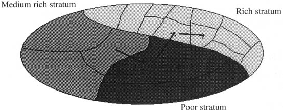