This chapter presents the equations used in program VIT. Its objective is to present a brief description of the methodology used in population dynamics to inform the user about the different options of the program. Therefore, this chapter is not a comprehensive review of population dynamics. For such review there are a number of basic books: Beverton&Holt (1957), Ricker (1975), Csirke (1980), Laurec & Le Guen (1981), Pitcher & Hart (1982), Pauly & Murphy (1982), Pereiro (1982), Gulland (1983), Sparre et al. (1989) and others.
The time unit is the year. This is the only variable with predetermined units. All other working units are fixed by the user through the values of the data and parameters. Therefore, during a given run of the program the same units must be used. For example, if the user desires to work in grams, all inputs requested by the program representing weight or biomass will have to be in these units (see table below). All output is then presented in this same units.
| Variable or Parameter | Magnitude | |
| Length | L | |
| Age | T | |
| Weight | M | |
| Catch | M T -1 | |
| Biomass | M | |
| Yield-per-recruit | M T -1 | |
| Biomass-per-recruit | M | |
| Growth: | L(inf) | L |
| k | T -1 | |
| t0 | T | |
| Length-weight: | a | M L-3 |
| b | ||
| Mortalities: | M, F, Z | T -1 |
In spite of what is said above it is not strictly necessary to use the year as a time unit. However, given that the equations work with ages and years, a change in time units may create problems: reconverting growth equations, desaggregating catches that may be affected by a seasonal component etc.. That is why it is not recommended to use any time unit other than the year.
VIT always work with grouped data, be it age or size. All data used corresponds to a histogram of absolute frequencies and the results make reference to this histogram. Each class corresponds to an interval of ages or sizes, which are all of equal width, except if there is a "plus" group. The "plus" group represents all individuals that are either bigger or older than the second to last class.
A data set will be made up of n classes. Let i be one of these classes, it is then possible to define the following symbols:
| Number of individuals at the beginning of class i | |
| Average annual number of individuals in class i | |
| Age of individual at the beginning of class i | |
| Average age of individuals in class i | |
| Length of individual at the beginning of class i | |
| Average length of individuals in class i | |
| Weight of individuals at the beginning of class i | |
| Average weight of individuals in class i | |
| Total and fishing mortality for class i | |
| Natural mortality (constant) | |
| Overall mean total and fishing mortalities | |
| Overall global fishing mortality | |
| Catch (in numbers) of individuals in class i | |
| Average annual biomass of individuals in class i |
In some equations the above symbols are used as functions instead of numeric values. In such case the symbols have no subscript, and may or may not indicate the independent variable. For example l or l(t) denote length as a function of time (age), whereas li denotes the length at the beginning of the size class i.
In section 5.5 the method for calculating average values is presented. The average lengths, weights and ages do not match, that is, whithin a class, the average weight or length are not the weight or length corresponding to the average age. This is because these functions are not linear.
The next class to i is symbolized with i+1. The difference in ages between the beginning of i and i+1 is a quantity commonly used and symbolized by:
![]()
Whenever the classes correspond to ages, almost always the time unit will be years,
therefore![]() .
.
The last class can be open or close, in the later case this class is denoted as plus group. In the example from section 4 the last class is closed and its limits are 83 cm and 85 cm. If it had been defined as Plus group the lower limit would remain at 83 cm, but the upper limit would be equal to L(inf), that is 95 cm. The age corresponding to this upper limit would then be infinity.
Individual growth is expressed by the Von Bertalanffy (1934) growth equation:
![]()
where L¥ , k and t0 are constants (these are respectively parameters L(inf), k and t0 from the growth equation)
The length-weight relationship is considered to be allometric (Huxley, 1924) and its expressed by a power function of the type:
![]()
where a and b are constants (respectively parameters a and b from the length-weight relationship).
The reconstruction of the virtual population can be done through the classic VPA or cohort analysis. Traditionally the former is used with age-structured data, and the later for both age and length structured data. For instance, the length-based cohort analysis (LCA, Jones 1982) is practically the only method for the analysis of length data, available in the common software. VIT allows for the four possible combinations between length and age and the VPA and cohort analysis equations.
To reconstruct the population according to the method that we denote as standard VPA (Gulland 1965), the usual population dynamic equations are used. For instance, the survival equation,
![]()
that can be expressed, for each class (in difference form) as
![]()
and the catch equation
![]()
The process starts with the last class. The number of individuals at the beginning of the last class is calculated using the catch equation with the terminal fishing mortality and the catch. Then, by replacing the survival equation in the catch equation, the following new expression is derived,
![]()
Given that Zi=Fi+M, the only unknown in the above equation is Fi. Because there is no analytical solution to this expression, an algorithm incorporating the method of the secant, is used to obtain an approximate solution. The tolerance of the convergence is 10-12, but it can be modified by the user through option 9 (hidden) from the Main menu (See section 3.4.9). If the algorithm has not converged after 50 iterations, the precision is reduced by one order of magnitude and a warning is shown on the screen. This process is repeated until a solution is found. Next time the subroutine that finds the approximate solution is used, the precision will again be equal to 10-12 (or equal to the last value given with option 9 in the Main menu during the same run of VIT).
Once Fi is known, the survival equation is used to calculate Ni. We have now solved for the class before last. The virtual population analysis is completed by repeating this process.
It uses the cohort equation from Pope (1972):
![]()
and the survival equation.
The process starts like in the previous case, by using the catch equation to calculate the number of individuals entering the beginning of the size class. Then with Pope's equation the number of individuals in the class before last is calculated. Next, the fishing mortality is derived by solving the survival equation. Once the class before last has been solved, the process is repeated until the population is fully reconstructed. Note that in this method all equations are solved analytically.
The equations that allow for the calculations of average values are the following:
Average annual numbers
![]()
Average age

Average length

Average weight

where
![]() , ti£ t<ti+1,
, ti£ t<ti+1, ![]() and
and ![]()
Given that the last integral cannot be solved analytically, the program uses numerical integration according to the Simpson rule and 20 classes. Note the change in variable (t for m ) to avoid improper integrals and disproportionate intervals to apply the Simpson rule in the presence of a plus group.
In addition to the above results, the program offers overall mortality values (if there is no plus group). For the overall total mortality, this computation is performed as:

and similarly for the overall mean fishing mortality, only substituting the Zs for Fs. According to the survival equation this is equivalent to weighting the mortalities according to the time during which they act. That is why in the presence of a plus group, these averages are not calculated. This is due to the fact that the plus group lasts eternally and, consequently, the overall total mortality would be equal to the mortality of the plus group. All these quantities allow summarizing the survival scheme of the cohort by considering the initial and final number of individuals. The later disregards the shape of the curve and the intermediate numbers resulting from the different fishing mortalities by class. In summary, these overall figueres do not reflect the catch distribution by class.
However, the program presents another quantity, the overall global fishing mortality that should not be confused with the overall mean fishing mortality mentioned above. The calculation of this other fishing mortality is based on the following concept:
The catch equation (section 5.4.1) can be rewritten as a function of the average annual number,
![]()
in a way that fishing mortality per class indicates the proportion of individuals caught in each class. This interpretation of fishing mortality can be extended to a pseudochort, given that the total catch
![]()
we can then define the overall global fishing mortality F* as,
![]()
or

This is an overall value that relates the total annual catch with the average number of individuals in the population. Note that it equates to an average fishing mortality weighted by the number of individuals. Therefore there is no problem with the plus group. It is important to note that this value cannot be applied to the survival equation because this equation requires average mortality. This overall value has been considered and often used by ICES working groups (Shepherd 1983).
VIT can work with a maximum of four fishing gears acting on the same resource. The treatment used for the m fishing gears is based on disaggregating the instantaneous rate of total fishing mortality for class i, Fi, into the mortalities exerted by each fishing gear j, Fi,j. In such a way that,
![]()
Actually, the VPA is done for all gears combined by calculating Fi for each class. After that, the Fi,j are estimated according to the next equation
![]()
where Ci,j indicates the number of individuals of class i captured by fishing gear j. The overall fishing mortalities for each gear (section 5.5), are calculated in the same way.
Once the population in numbers has been reconstructed, the transformation to biomass is done from the average numbers and weights for each class
![]()
(see section 5.5). The information provided by these calculations is very useful, and the w7219e of the population in biomass terms is very illustrative.
From these results, it is possible to obtain the critical ages and lengths (those corresponding to the points where the cohort reaches the maximum in biomass), for the virgin stock and for the present level of exploitation. To calculate the later the only requirement is to locate the class which provided the greatest biomass. In the case of the virgin stock, the critical age is obtained from the following expression:
![]()
analytically obtained from the maximum biomass of the virgin stock as a function of time
![]()
where N(t) is derived from the survival equation (section 5.4.1) in the absence of fishing, that is,
![]()
and w(t) is derived from the growth equations (section 5.3). Finally, the critical length for the virgin stock is calculated by substituting the value of the critical age tc in the Von Bertalanffy growth equation (section 5.3).
Yield-per-recruit analysis allows the user to get a more global vision of the population under study. Recruitment is defined as the number of individuals at the beginning of the first class, and yield as the total weight of the catch. Therefore, the yield-per-recruit is obtained by dividing the total weight of the catch by the number of recruits calculated from the VPA. However, because Y/R analysis attempts to investigate how this quantity changes as a function of fishing effort, there is a need for an alternative expression that incorporates fishing effort. The formula used in VIT is derived from the catch equation, expressed as a function of the average number of individuals per class (section 5.5):
![]()
The Y/R value obtained from this expression is equivalent to the one obtained by dividing the catch by the recruitment. It is therefore compatible with the catch equation. In comparison with other alternative expressions presented below, the above is said to be the exact formula for Y/R.
Note that the above expression requires for each class, the average number of individuals and the average weight (See section 5.5) These values and the fishing mortality vector are obtained from the VPA.
The usefulness of the yield-per-recruit analysis resides precisely, on observing its behavior as fishing effort varies. In order to do this the program introduces a factorf , that multiplies fishing effort, and that is interpreted as an effort factor. If for example the values 0, 0.5, and 2, are given to this factor, they will represent fishing efforts equal to the absence of fishing, half and double of the present fishing effort.
According to the above, the correct Y/R is expressed as a function of the fishing effort factor f ,
![]()
Note that for each value of f the average numbers and weights have to be recalculated with a new VPA. This makes this analysis very slow. It is possible to use option 3 in the Y/R menu to simplify these calculations and make them approximative but quicker (section 3.4.5.3):
One of the options, "with initial weights", is based on the equation
![]()
that differs from the Y/R equation previously stated as the correct one, in
that it uses the weights wi, at the beginning of the class rather than
the average weights![]() . This option
is included to compare the results of VIT with those of other programs that use equation
above to save time, for example Hightower (1986). However, unless that is the purpose of
the analysis, its use is not recommended because it significantly underestimates Y/R.
. This option
is included to compare the results of VIT with those of other programs that use equation
above to save time, for example Hightower (1986). However, unless that is the purpose of
the analysis, its use is not recommended because it significantly underestimates Y/R.
The other option, "With mean weights from current VPA", uses for all calculations a single average weight vector: that calculated in the last run of VPA. Therefore the Y/R values are only exact for f =1. The values for f <1 are underestimated and those for f >1 are overestimated. The program runs much faster because it does not need to recalculate the average weights per class for each value of f , and the results are only slightly less precise. This may be useful for the initial trial runs, but it is recommended that the correct equation be used in the final analyses.
This option performs an analysis in the absence of equilibrium. It is the only part of the program where equilibrium is not assumed. Basically, it consists in simulating the evolution of the population when either the fishing mortality or recruitment are not constant.
The functioning mechanism is as follows: it starts with the equilibrium population structure generated by the VPA - consisting in vectors with the number of individuals at the beginning of each class and a fishing mortality per class vector. This is the initial equilibrium state at the beginning of the process. The user indicates the number of years for the simulation (maximum 40), then the fishing mortality vector and the recruitment model can be modified by the user.
This analysis can be used, not only for studying the evolution of the fishery in the presence of changes in recruitment or the exploitation pattern, but also to study the sensitivity of the stock to recruitment (eg. Pallarés and Pereiro 1990). It is for this purpose that the program allows for the introduction of stochastic recruitment.
The modification of fishing effort can be done in two ways (options 1 and 2 in A in section 3.4.6).
The first option (A=1), consists in multiplying all the elements in the F vector by a single factor. In such case the proportions by class are maintained.
The second option (A=2), consists in substituting the F vector generated from the VPA by a new vector (where the proportions by class do not have to be maintained). With this process it is possible to simulate a change in gear selectivity.
The two changes above can also be done in two different ways (options 1 and 2 in B, section 3.4.6):
Perform the change in a single year (the first one in the simulation), and maintain through the process the new fishing mortalities (option B=1), or introduce a new F vector for each year of the simulation (option B=2).
Therefore the user has four possibilities to modify the effort within the transition analysis: (A=1, B=1), (A=1, B=2), (A=2, B=1) and (A=2, B=2).Once all years requested have been simulated, the program presents the equilibrium results for the last set of Fs entered.
The user of VIT has to decide on the stock-recruitment model to be used, and whether to add stochastic variability to the recruitment.
The default option is constant recruitment equal to 1, however it is also possible to use the B&H (Beverton & Holt, 1957) and the Ricker model (Ricker, 1954). The choice of one of the three recruitment model options (constant, B&H, or Ricker) is independent of the choice on imposing stochasticity.
The initial hypotheses state that the stock is in equilibrium and that, at the level of spawning stock biomass-per-recruit calculated by the VPA, recruitment is equal to 1. This limits the number of values that the stock-recruitment parameters can take. The stock-recruitment curves, R vs S, where R is the recruitment and S the spawning stock biomass (SSB) have to go through R=1 when S takes the value of spawning biomass calculated by the VPA.
According to Beverton and Holt, the equation that relates stock and recruitment is:

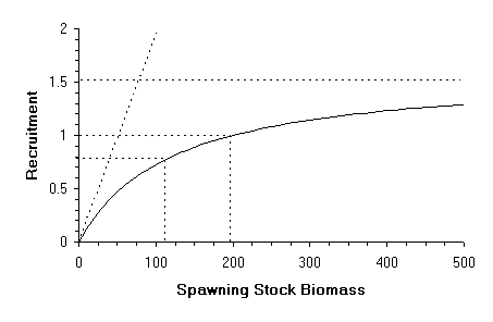
Graphically (Figure 1) this represents a monotonous, asymptotic function that goes through the origin. The value of the asymptote is R=1/a and the slope at the origin is 1/b. There are three different ways that can help the user determine the parameters of the above equation (remember that for the current S, R has to be equal to 1):
1 Fixing the value of the spawning stock biomass to give a recruitment value equal to half of the asymptote. This value S1/2 has to be smaller than the spawning stock biomass value calculated in the VPA. In this case a = S/(S+S1/2) and b = S(1-a).
2 Fixing the value of the slope at the origin (which has to be greater than 1/S). The parameter b is the inverse of that slope and a = 1-b/S.
3 Fixing the value of the asymptote (has to be greater than 1), a will be the inverse of the asymptote and b = S(1/a).
Figure 1
Graphical example of a Beverton & Holt stock-recruitment curve indicating: the asymptote, the slope at the origin, the values of spawning stock biomass-per-recruit corresponding to a recruitment of 1 and to a recruitment of half of the asymptote.
According to Ricker the equation which relates stock and recruitment is:
![]()
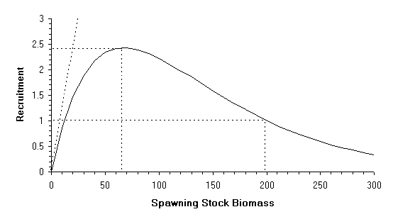
Graphically this is a curve that passes through the origin (Figure 2), that presents a maximum and is asymptotic to zero (R=0 when S ® ¥ ). The maximum of the curve is at R = a /b e and S=1/b . There are two different ways that can help the user to determine the parameters of the above equation (remember that for the present S, R has to be equal to 1):
1 Fixing the value of S which gives the maximum recruitment (SM). Then b = 1/SM and a = 1/(S exp(-b S)).
2 Fixing the value of the slope at the origin, which is equal to a . Then the other parameter is b = Ln(a S)/S.
Note that in this case the option of calculating parameters by selecting a value of spawning stock which gives half of the maximum recruitment is not offered as it was in the Beverton and Holt model. This is because the Ricker model is not monotonously increasing and has an asymptote of zero. Consequently there are two values of spawning stock corresponding to each value of recruitment between zero and the maximum (Figure 2).
Figure 2
Graphical example of a Ricker stock-recruitment curve, indicating the maximum, the slope at the origin and the value of spawning stock biomass per recruit corresponding to a recruitment of 1 (R=1).
Whichever stock-recruitment model is used, it is possible to generate stochastic recruitment. To make the computations compatible with a recruitment of 1 (R=1), this stochastic component is lognormally distributed with mean 1. Therefore, if the variance is zero, recruitment is equal to 1 and if the variance is greater than 0, recruitment is never negative (something possible if, for example, a normal distribution had been chosen).
A lognormal distribution with mean E(x) and variance Var(x) corresponds to a normal distribution with mean m and variance s 2. The functions that relate these two quantities are:

and
![]()
That is why, to obtain random numbers distributed as a lognormal with mean E(x)=1 and variance Var(x), fixed by the user, the program proceeds to calculate random numbers from a normal distribution N(m ,s 2).
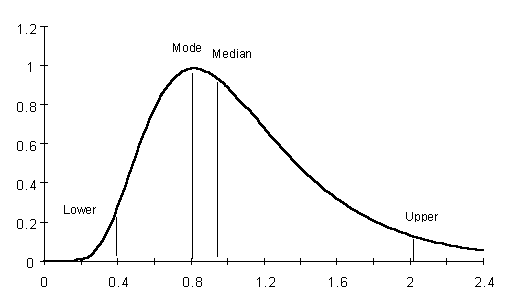
The lognormal distribution has the mean and variance not independent. To help the user set a variance the program provides some on-line help on the mode and 95% confidence intervals of the distribution for a given variance (See section 3.4.6). The next figures, 3 and 4, provide examples of the properties of this distribution.
Figure 3
Examples of lognormal distributions. The 6 distributions have the same mean (=1) and differ in their variance whose value is indicated next to each curve. Note that the greater the variance, the greater the asymmetry of the curve.
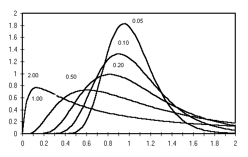
Figure 4
Graphic of a lognormal distribution with mean of 1 and variance of 0.2 with an indication of the mode, median, and the lower and upper limits of the 95% confidence intervals.
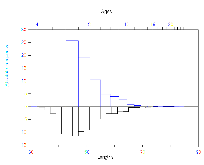
The conversion of lengths to ages is done by superimposing the abscissa axis of the length frequency histogram to the corresponding age axis. Ages are calculated according to the Von Bertalanffy equation and the length frequencies are divided to each age interval proportionally. This is the procedure known as slicing. See figure 5 below.
Figure 5
Example of a transformation from lengths to ages. The length frequency histogram is in the lower part, and the resulting age frequency histogram is in the upper part. Note how the age scale is not linear because it has been derived from the growth equation.
