![]()
![]()
![]()
Effects of surface mulches
Intercropping
Small areas of vegetation
Management induced environmental stress
This chapter discusses various types of factors that may cause the values for Kc and ETc to deviate from the standard values described in the Chapters 6 and 7. These factors refer to the effects of surface mulches, intercropping, small areas of vegetation and specific cultivation practices.
This chapter is intended to serve as a resource for situations where cultivation practices are known to deviate from those assumed in Tables 12 and 17, but where estimates of Kc and ETc are still necessary. This chapter is by no means exhaustive. The intent is to demonstrate some of the procedures that can be used to make adjustments to Kc to account for deviations from standard conditions.
Mulches are frequently used in vegetable production to reduce evaporation losses from the soil surface, to accelerate crop development in cool climates by increasing soil temperature, to reduce erosion, or to assist in weed control. Mulches may be composed of organic plant materials or they may be synthetic mulches consisting of plastic sheets.
Plastic mulches generally consist of thin sheets of polyethylene or a similar material placed over the ground surface, especially along the plant rows. Holes are cut into the plastic film at plant spacings to allow the plant vegetation to emerge. Plastic mulches can be transparent, white or black. Colour influences albedo mainly during the early stages of the crop. However, as the intention is to use a simple procedure for adjusting Kc for mulched crops, no distinction is made between the different types of plastic mulches.
Plastic mulches substantially reduce the evaporation of water from the soil surface, especially under trickle irrigation systems. Associated with the reduction in evaporation is a general increase in transpiration from vegetation caused by the transfer of both sensible and radiative heat from the surface of the plastic cover to adjacent vegetation. Even though the transpiration rates under mulch may increase by an average of 10-30% over the season as compared to using no mulch, the Kc values decrease by an average of 10-30% due to the 50-80% reduction in soil evaporation. A summary of observed reductions in Kc, in evaporation, and increases in transpiration over growing seasons is given in Table 25 for five horticultural crops. Generally, crop growth rates and vegetable yields are increased by the use of plastic mulches.
TABLE 25. Approximate reductions in Kc and surface evaporation and increases in transpiration for various horticultural crops under complete plastic mulch as compared with no mulch using trickle irrigation
|
Crop |
Reduction 1 in Kc (%) |
Reduction 1 in evaporation (%) |
Increase 1 in transpiration (%) |
Source |
|
Squash |
5-15 |
40-70 |
10-30 |
Safadi (1991) |
|
Cucumber |
15-20 |
40-60 |
15-30 |
Safadi (1991) |
|
Cantaloupe |
5-10 |
80 |
35 |
Battikhi and Hill (1988) |
|
Watermelon |
25-30 |
90 |
-10 |
Battikhi and Hill (1986), Ghawi and Battikhi (1986) |
|
Tomato |
35 |
not reported |
not reported |
Haddadin and Ghawi (1983) |
|
Average |
10-30 |
50-80 |
10-30 |
|
1 Relative to using no mulch
Single crop coefficient, Kc
To consider the effects of plastic mulch on ETc, the values for Kc mid and Kc end for the horticultural crops listed in Table 12 can be reduced by 10-30%, depending on the frequency of irrigation (use the higher value for frequent trickle irrigation). The value for Kc ini under mulch is often as low as 0.10. When the plastic mulch does not entirely cover the soil wetted by the drip emitters, or where substantial rainfall occurs, then the reduction in Kc mid or Kc end will be less, in proportion to the fraction of wet surface covered by the mulch.
Dual crop coefficient, Kcb + Ke
When estimating basal Kcb for mulched crops, less adjustment is normally needed to the Kcb curve, being of the order of a 5-15% reduction in Kcb, as it is generally understood that the 'basal' evaporation of water from the soil surface is less with a plastic mulch, though the transpiration is increased. The effect on Kcb could be greater in some situations and with some types of low density crops. Local calibration of Kcb (and Kc) for use with mulch culture is encouraged.
When calculating the soil evaporation coefficient Ke with plastic mulch, the fw should represent the relative equivalent fraction of the ground surface that can contribute to evaporation through the vent holes in the plastic cover and to the fraction of surface that is wetted, but is not covered by the mulch. The effective area of vent holes is normally two to four times the physical area of the vents (or even higher) to account for vapour transfer from under the sheet.
Organic mulches are often used with orchard production and with row crops under reduced tillage operations. Organic mulches may consist of unincorporated plant residues or foreign material imported to the field such as straw. The depth of the organic mulch and the fraction of the soil surface covered can vary widely. These two parameters will affect the amount of reduction in evaporation from the soil surface.
EXAMPLE 45. Effects of surface mulch
|
A plastic mulch is placed over cucumbers under drip irrigation. The mulch is clear plastic covering the entire field surface, with small openings at each plant. Adjust both the mean and basal Kc values for this crop to reflect the presence of the mulch. |
|
From Table 12, Kc ini, Kc mid and Kc end for fresh market cucumbers have values equal to 0.4, 1.0 and 0.75. As the plastic mulch is continuous with only small vents at each plant, the Kc ini is assumed to be only 0.10 (this value should be adjusted upward if precipitation occurs). The Kc mid and Kc end values are estimated as: Kc mid = 0.85 (1.0) = 0.85 where the 0.85 multipliers are derived from Table 25 and reflect an assumed 15% reduction in ETc due to the mulch, assuming an approximately weekly irrigation frequency. From Table 17, the values for Kcb ini, Kcb mid, and Kcb end are 0.15, 0.95 and 0.7 for this same cucumber crop. The Kcb ini is assumed to be similar to the Kc ini for mulched cover and is therefore set equal to 0.10. The Kcb mid and Kcb end values are estimated to be reduced by 10% so that: Kcb mid = 0.9 (0.95) = 0.86 These basal values are similar to the adjusted values for Kc. This is expected as evaporation from the mulch covered surface can be ignored. Additional adjustment to these Kc values to account for climate is necessary using Eq. 62 and 70. |
|
The values for mean Kc and Kcb are similar with values of 0.10 for the initial stage, 0.85 for the mid-season stage and 0.64 at the end of the late season stage. |
Single crop coefficient, Kc
A general rule when applying Kc from Table 12 is to reduce the amount of soil water evaporation by about 5% for each 10% of soil surface that is effectively covered by an organic mulch.
For example, if 50% of the soil surface were covered by an organic crop residue mulch, then the soil evaporation would be reduced by about 25%.
· In the case of Kc ini, which represents mostly evaporation from soil, one would reduce Kc ini by about 25% in this situation.· In the cases of Kc mid and Kc end, one would reduce these values by 25% of the difference between (Kc mid - Kcb mid) and (Kc end - Kcb end) from Tables 12 and 17. Generally, the differences between values in Tables 12 and 17 are only 5-10% so that the adjustment to Kc mid and Kc end to account for an organic mulch may not be very large.
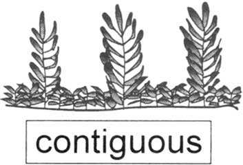
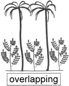
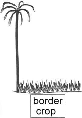
FIGURE 45. Different situations of intercropping
Dual crop coefficient, Kcb + Ke
When applying the approach with a separate water balance of the surface soil layer, the magnitude of the evaporation component (Ke ETo) should be reduced by about 5% for each 10% of soil surface covered by the organic mulch. Kcb is not changed.
These recommendations are only approximate and attempt to account for the effects of partial reflection of solar radiation from residue, microadvection of heat from residue into the soil, lateral movement of soil water from below residue to exposed soil, and the insulating effect of the organic cover. As these parameters can vary widely, local observations and measurements are required if precise estimates are required.
Intercropping refers to the situation where two different crops are grown together within one field. For the estimation of the crop coefficient, a distinction is made between (Figure 45):
· Contiguous vegetation, where the canopies of the two crops intermingle at some height (e.g., corn and beans intercropping);· Overlapping crops, where the canopy of one crop is well above that of the other so that the canopies cannot be considered to be contiguous (e.g., date trees overlapping pomegranate trees at an oasis); and
· Border crops, where tall crops such as windbreaks border fields of shorter crops, or high trees border a field crop.
There is an upper limit to the energy available to evaporate water. This is represented by Kc max (Equation 72 of Chapter 7) for all crops in cultivated fields larger than 3-5 ha:
(72)
where h is the height for the taller crop. Under all conditions when combining crop coefficients for multiple crops, Kc should be constrained by this upper bound (Kc £ Kc max).
Where the taller crop has canopy foliage that extends down to the same elevation as that of the top of the shorter crop, the vegetation canopy can be considered to be contiguous. For example, in Africa and South America, maize and beans are frequently intercropped as contiguous vegetation, with one row of maize planted per one or more rows of beans. Another example is the cultivation of five to seven rows of wheat intercropped with three rows of maize in many areas of China.
Similar ground cover
Where the leaf area or fraction of ground covered by the vegetation (fc) is similar for each crop, the Kc in Tables 12 and 17 for the taller crop (if this Kc is higher) can be taken to represent the entire field. The taller crop will act in some sense as a clothesline so that Kc (and ETc) for the taller crop per unit of ground area is increased over that given in Table 12 or 17. However, the Kc (and ETc) for the shorter crop will be reduced due to the windbreak effect by the taller crop. As a result, the Kc for the field as a whole may be similar to the weighted average of the Kc values for the two crops from Tables 12 and 17, or, the total Kc may more closely follow the Kc predicted for a field sown entirely to the taller crop (Kc field » Kc taller crop). Yields for the shorter crop may be reduced relative to those for single cultivar production due to the effects of shading by the taller crop and the competition for soil water.
Different ground cover
Where the fractions of ground covered by each crop are different, the Kc for an intercropped field can be estimated by weighting the Kc values for the individual crops according to the fraction of area covered by each crop and by the height of the crop:
(104)
where f1 and f2 are the fractions of the field surface planted to crops 1 and 2, h1 and h2 are the heights of crops 1 and 2, and Kc1 and Kc2 are the Kc values for crops 1 and 2.
Where intercropping entails overlapping of spacings, the canopy of one crop is well above the other. This is the case, for example in southern California, where citrus trees are planted in date palm groves. Where a normal dense spacing is used for both the dates and for the citrus trees, the Kc may increase as the density of the combined vegetation increases, proportional to the increase in LAI (Example 47), with maximum Kc constrained by either Kc max (Equation 72) or by Kcb full (Equations 99 and 100) unless the total field area is small so that there is an additional clothesline or oasis effect as discussed in the next section.
EXAMPLE 46. Intercropped maize and beans
|
Determine the representative Kc mid for a situation where a single 1 m wide row of maize is grown for each 2 m of squash, where RHmin » 45% and u2 » 2 m/s. |
|
From Table 12, the Kc mid and h for maize is 1.20 and 2 m and the Kc mid and h for squash is 0.95 and 0.3 m. No correction is needed for climate. The representative Kc mid can be obtained by weighting the individual Kc mid values according to the fraction of the field surface allocated to each crop (f1 » 0.3 for maize and f2 » 0.7 for squash) and according to the heights of the crops as (Eq. 104):
Values can be obtained for daily Kc in a similar manner by constructing individual Kc curves and then weighting interpolated values from the individual Kc curves for any specific day using Eq. 104. |
|
The crop coefficient for the mid-season and entire field is 1.14. |
Where tall crops such as windbreaks or date palms border fields of shorter crops, the upper storey of the taller crop can intercept extra sensible heat energy from the air stream. Under these conditions, the Kc is weighted according to the areas for each crop. However, prior to the weighting, the Kc for the border crop, if taller than the field (interior) crop, should be adjusted for potential clothesline impact (next section).
Areas surrounded by vegetation having similar roughness and moisture conditions
Clothesline and oasis effects
Natural vegetation and some subsistence agriculture frequently occurs in small groups or stands of plants. The value for Kc for these small stands depends on the type and condition of other vegetation surrounding the small stand.
In the majority of cases for natural vegetation or for non-pristine agricultural vegetation, the value for Kc must adhere to upper limits for Kc of approximately 1.20-1.40, when the areal expanse of the vegetation is larger than about 2000 m2. This is required as ET from large areas of vegetation is governed by one-dimensional energy exchange principles and by the principle of conservation of energy. ET from small stands (< 2000 m2) will adhere to these same principles and limits only where the vegetation height, leaf area, and soil water availability are similar to that of the surrounding vegetation.
EXAMPLE 47. Overlapping vegetation
|
A 20 ha date palm grove in Palm Desert, California, the United States has a tree spacing of 6 m. Interplanted among the rows of palms are small orange trees (50% canopy) on a 6 m spacing. The palm and citrus trees are 3 m from one another in the rows. Height of the palms is 10 m and height of the citrus is 3 m. The canopy foliage of the palms is well above that of the citrus so that the canopies cannot be considered contiguous. Mean average RHmin during the mid-season is 20% and u2 = 2 m/s. The Kc mid from Table 12 for dates is 0.95 and when adjusted for humidity and wind using Eq. 62 is Kc mid = 1.09. The Kc mid from Table 12 for citrus having 50% canopy with no ground cover is 0.60 and when adjusted for humidity and wind using Eq. 62 is Kc mid = 0.70. |
|
The interplanting of citrus among the date palms has increased the total leaf area of the orchard so that ETc for the combined planting (palms and citrus together) will be greater than for either planting alone. The estimated combined Kc mid will be estimated as a function of the increase in total LAI. First the LAI values of the individual plantings are estimated by inverting Eq. 97 to solve for LAI:
where Kc min is the minimum basal Kc for bare soil (a 0.15 to 0.20) and Kcb full is the maximum mid-season Kc expected for the crop if there were complete ground cover, calculated using Eq. 99. Based on Eq. 99, with h = 10 m for the date palms and h = 3 m for the citrus, the Kcb full values for the two crops, assuming complete ground cover for each, are Kcb full = 1.34 for palms and Kcb full = 1.30 for citrus (using RHmin = 20% and u2 = 2 m/s). These estimates ignore effects of any unique stomatal control. Therefore, using the above equation, the effective LAI values of the date palms and citrus are estimated to be approximately: LAIpalms = -1.4 ln[1 - (1.09 - 0.15)/(1.34 - 0.15)] = 2.2 Therefore, the effective LAI for the date palm-citrus combination is estimated to be approximately LAIcombined = LAIpalms + LAIcitrus = 2.2 + 0.9 = 3.1. |
|
The increase in Kc mid for the date palm orchard resulting from the increase in LAI from the interplanting of citrus is estimated using a ratio of the LAI-based function introduced in Eq. 97. This results in the relationship:
where LAIcombined is the LAI for the two intercropped plantings combined and LAIsingle crop is the LAI for the taller, single crop. Kc mid single crop is the mid-season Kc for the taller, single crop (in this case the date palms). In this application, the above equation is solved as:
Therefore, the Kc mid estimated for the complex of date palms and citrus together is 1.23. This value is compared with the maximum expected Kc based on energy limitations, represented by Kc max of Eq. 72 which in this case for h = 10 m is Kc max = 1.34. Because Kc mid < Kc max (i.e., 1.23 < 1.34), the Kc mid = 1.23 is accepted as the approximate estimate of the Kc mid for the intercropped field. |
Under the clothesline effect, where vegetation height is greater than that of the surroundings (different roughness conditions), or under the oasis effect, where vegetation has higher soil water availability than the surroundings (different moisture conditions), the peak Kc values may exceed the 1.20-1.40 limit. The user should exercise caution when extrapolating ET measurements taken from these sorts of vegetation stands or plots to larger stands or regions as an overestimation of regional ET may occur.
Small expanses of tall vegetation that are surrounded by shorter cover can exhibit a clothesline effect. This occurs where turbulent transport of sensible heat into the canopy and transport of vapour away from the canopy is increased by the 'broadsiding' of wind horizontally into the taller vegetation. In addition, the internal boundary layer above the vegetation may not be in equilibrium with the new surface. Therefore, ET from the isolated expanses, on a per unit area basis, may be significantly greater than the corresponding ETo computed for the grass reference. Examples of the clothesline or oasis effects would be ET from a single row of trees surrounded by short vegetation or surrounded by a dry non-cropped field, or ET from a narrow strip of cattails (a hydrophytic vegetation) along a stream channel. Kc values up to and exceeding two have been recorded for such situations.
Where ET estimates are needed for such small, isolated expanses of vegetation surrounded by shorter cover (clothesline effect) or dry land (oasis effect), then the Kc may exceed the grass reference by 100% or more. Estimates of Kc for the expanses of vegetation should contain u2, RHmin and h parameters to adjust Kc values, and parameters expressing the aridity of the surrounding area, the general width of the vegetation stand and the ability of the wind to penetrate into the vegetation. The equation should also consider the LAI of the vegetation to account for the ability of the vegetation to conduct and transpire the amount of water demanded by the clothesline/climatic condition. An upper limit of 2.5 is usually placed on Kc to represent an upper limit on the stomatal capacity of the vegetation to supply water vapour to the air stream under the clothesline or oasis conditions. For vegetation with a great leaf resistance, such as for some types of desert vegetation or trees, the upper limit should be multiplied by a resistance correction factor, Fr, calculated in Chapter 9 using Equation 102.
Figure 46 presents example curves of Kc for small areas of vegetation versus vegetation stand width, for conditions where u2 = 2 m/s, RHmin = 30%, vegetation height = 2 m, and LAI = 3. The upper curve represents conditions where the specific vegetation is surrounded by dead vegetation, dry bare soil, or even gravel or asphalt. In this situation, large amounts of sensible heat are generated from the surrounding area due to the lack of ET. Some of this sensible heat is advected into the vegetation downwind. The lower curve represents conditions where the vegetation is surrounded by well-watered grass. In this situation, there is much less sensible heat available from the surrounding area to increase ET (and Kc) of vegetation downwind. The influence of the aridity of the surroundings on the Kc for a small expanse is apparent. The two curves shown will change with changes in u2, RHmin, h, and LAI. The user is cautioned that Figure 46 provides only general estimates of Kc under clothesline and oasis conditions. These estimates should be verified where possible using valid local measurements.
FIGURE 46. Kc curves for small areas of vegetation under the oasis effect as a function of the width of the expanse of vegetation for conditions where RHmin = 30%, u2 = 2 m/s, vegetation height (h) = 2 m and LAI = 3
ET estimates from large expanses of vegetation or from small expanses of vegetation that are surrounded by mixtures of other vegetation having similar roughness and moisture conditions should almost always be less than or equal to 1.4 ETo, even under arid conditions.
For tall wind breaks, such as single rows of trees, an approximate estimate for Kc is:
(105)
where
Fr stomatal resistance correction factor (Equation 102)
hcanopy mean vertical height of canopy area [m]
Width width (horizontal thickness) of the windbreak [m]
The Kc = 2.5 limit imposed in Equation 105 represents an approximate upper limit on ETc of trees per unit ground area. However, this value has large uncertainty. Because availability of soil water may limit evapotranspiration from wind breaks, a soil water balance and calculation of the Ks stress factor should be conducted.
Many agricultural crops are intentionally water stressed during specific crop growth periods to encourage particular crop characteristics. The water stress is initiated by withholding or by reducing irrigations. In situations where this type of cultural management is practised, the Kc should be reduced to account for the reduction in evapotranspiration.
Environmental stress from soil water shortage, low soil fertility, or soil salinity can cause some types of plants to accelerate their reproductive cycle. In these situations, the length of the growing season may be shortened, particularly the mid-season period. Stress during the development period may increase the length of that period. Therefore, the length of the mid-season, Lmid, and perhaps the lengths of the development and late seasons may need to be adjusted for environmentally stressed or damaged vegetation. Local research and observation is critical to identify the magnitudes and extent of these adjustments. Some examples of modifications to Kc and to lengths of growing periods are described below.
Some forage crops such as alfalfa that are grown for seed production are intentionally water stressed to reduce the amount of vegetation and to encourage increased production of flowers and seed. In areas subject to freezing winters, the reduction in Kc for deep rooted crops such as alfalfa depends upon the amount of water made available from precipitation during the dormant (winter) season and upon the amount of rainfall and limited irrigation during the growing season. Therefore, the effects of the intentional stress on the values for Kc should be modelled using the basal crop procedure presented in Chapter 7 and the Ks coefficient and water balance procedure presented in Chapter 8.
In cotton production, soil water stress may be initiated during the development period to delay flower development and to encourage boll development. This practice retards the growth rate of the cotton plant and delays the date of full cover. For cotton, the attainment of full cover and the beginning of the mid-season generally occurs when the LAI reaches approximately three. When soil water stress and growth retardation is practised, full cover may occur after the beginning of flowering. The effect of stress during the development period on ETc can be incorporated into the Kc curve by extending the length of the development period into the mid-season period. The length of the total season generally remains the same.
Sugar beets are frequently managed to initiate mild soil water stress during the late season period to dehydrate roots and concentrate sugars. A terminal irrigation may be needed just prior to harvest to assist in root extraction. When this type of water stress is practised, the value for Kc end is reduced from 1.0 to 0.6 (Table 12, Footnote 5).
Coffee plants are often intentionally water stressed to reduce vegetation growth and to encourage development of berries. Under these conditions, Kc values from Table 12 should be reduced. In addition, coffee fields may be bordered by trees that serve as windbreaks. The effect of windbreaks is to reduce the Kc of the coffee plants due to a reduction in wind and solar radiation over the plants. The reduction in Kc could be significant where windbreaks are tall and frequent. However, the Kc for the entire field area, including the windbreaks, may be increased by the presence of the trees, relative to the values for Kc for coffee shown in Table 12, due to increased total leaf area of the coffee-tree combination and the increased aerodynamic roughness.
Initiation and development of new leaves on tea plants often occurs following the start of the rainy season. During the dry season, initiation of new leaves is slow or non-existent. The transpiration from older leaves is lower than for new leaves due to effects of leaf age on stomatal conductance. Therefore, the Kc, when leaves have aged (more than 2-3 months old), will be perhaps 10-20% lower than shown in Tables 12 and 17. Similar to coffee, tea fields may be bordered by trees that serve as windbreaks. The effect of windbreaks is to reduce the Kc of the tea plants, but to potentially increase the Kc for the entire plantation, as described for coffee.
Growers may increase spacings of olive trees under rainfed conditions in areas with less rainfall. This is done to increase the ground area per tree that contributes infiltrated rain to transpiration of the tree. For example, in Tunisia, the spacing of olive trees changes from the north to the south, in proportion to annual rainfall. The tree spacing influences the Kc for the crop (Example 43).
![]()
![]()
![]()