5. GLOBAL ACCURACY BOUNDARIES

5.1 The feasible domain of A-curves for flat and convex populations

According to proposition 4.3 the WOMA of a flat population constitutes a lower limit for all convex populations and an upper limit for all concave populations with size N. In this section it will be shown that this limit has value:

Let us assume a flat(=equidistant) population with elements , size N and mean . It is clear that each of its elements can be written as:

with i=1,2,...,N

Since the population is symmetrical the worst accuracy curve will be formulated by working either from left to right or from right to left. We choose to work from left to right with sample sizes 1,2,...,N. In this manner and by using the property , the sample mean at each size n will be:

and, recalling that , the resulting accuracy will be:

By using the notation , then n=Nx and the above expression can be written as:

Expression (5.2) represents a "Global Line" G(x) of the general form:

where the intercept a is given by the formula:

From (5.2) it follows that when x starts from its minimum the line G(x) takes the value:

while for the maximum x=1 it becomes 1. Therefore the area formed by the line G(x) and the interval [, 1] on the x-axis (also representing the WOMA of the flat population), will be given by:

which explains the value of given in (5.1).

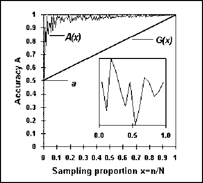
Fig. 5.1. Feasible domain of A-curves for non concave populations (N=200)

Figure 5.1 illustrates an example of a global boundary G(x) for all A-curves of convex and flat populations with size N=200. In this particular example the target population is flat and its distribution is shown in the small graph inside the plot.

It is easy to verify that the expression (5.4) for the intercept a is equivalent to:

with given as in (5.1).

In fact by substituting in (5.5) the value we obtain:

thus resulting in the same expression for a as in (5.4).

As it will be seen in Section 5.4 this observation will be useful in summarizing the formulae for the global boundaries G(x) and using a single formula for a.

5.2 The feasible domain of A-curves for all population categories

In the previous Section it was shown that there exists a lowest WOMA for all flat and convex population of the same size, and this lower limit has the value given in expression (5.1). The question now arises as to whether there exist fixed feasible domains for all A-curves in populations of the same size, that is including all three population categories: convex, flat and concave.

In response to this question it will be demonstrated that for all populations of a given size N, the feasible domain of all A-curves has a lower boundary corresponding to a WOMA with value:

Proposition 4.3 stated that by making a population more concave, its new WOMA becomes lower than the original one. The concluding paragraph of 4.3 also stated that by using the same transformation process for concave populations there will be a point at which all population elements will become extreme values 0 and 1. The question then arises as to which proportions of zero and non-zero elements will result in the lowest possible WOMA.

It will be presently shown that this proportion, denoted by r, will be given by:

If M is the unknown number of zero elements then the ratio r will be . The number of elements with value 1 will be (N-M) and the population mean will thus be:

We can now assume that which is equivalent to r<0.5 and implies that the population mean 1-r is found to the right of 0.5 (the opposite assumption for M would lead to the same results by means of a symmetrical approach).

We then proceed to the formulation of the worst PSA as described in Section 3.4 by considering four different sampling patterns depending on the sample size n.

Sampling pattern 1

In this first pattern the sample size n varies between 1 and M. All left-to-right sample means will be zero and all right-to-left sample means will be 1.

Evidently, the worst accuracy will correspond to since, according to (5.8) and the assumption that r<0.5, these sample means will be more distant from m = 1-r than . The corresponding worst accuracy will thus be:

and it will be constant when n varies between 1 and M.

A second observation is that by referring to the accuracy plot with the independent variable x taking values from to , the area of the rectangle formed by the horizontal line W=r and the interval [, r] on the x-axis will be:

Sampling pattern 2

In this second sampling pattern the sample size n varies between M and . The left-to-right sample means and worst accuracy are computed as:

The right-to-left sample means and worst accuracy are computed as:

It is easy to verify that . In fact, the relationship is equivalent to which is true because and in the current sampling pattern it was assumed that .

It has thus been shown that in the second sampling pattern the worst accuracy W will still be computed by using left-to-right samples and according to expression (5.10).

By referring again to the accuracy plot with the independent variable x taking values from to , the area formed by the curve W and the interval [r, 0.5] on the x-axis will be:

Sampling pattern 3

Here the sample size n varies between and N-M. The left-to-right and right-to-left sample means are computed as in sampling pattern 2 and the resulting worst accuracy values are given by expressions (5.10) and (5.11). However, in this pattern we have which is equivalent to and implies that in the third sampling pattern the worst accuracy W will be constant and equal to 1-r.

By referring to the accuracy plot with the independent variable x taking values from to , the area of the rectangle formed by the horizontal line W=1-r and the interval [0.5, 1-r] on the x-axis will be:

Sampling pattern 4

Finally, in the fourth sampling pattern the sample size n varies between N-M and N. The left-to-right sample means and worst accuracy are computed as:

The right-to-left sample means and worst accuracy are computed as:

Next step is to test that . This is equivalent to:

, or

, or

, or

The last relation is true because 1-2r>0 and . This observation implies that in the fourth sampling pattern the worst accuracy W should be formulated by using right-to-left samples and according to expression (5.14).

By referring to the accuracy plot with the independent variable x taking values from to , the area formed by the curve W and the interval: [1-r, 1] on the x-axis will be:

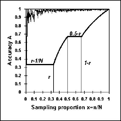
Fig. 5.2. The mixed curve W(x) representing the lowest WOMA for all populations with size N.

Figure 5.2 illustrates the process of formulating the mixed curve W(x) describing the lowest WOMA of all population categories with the same size N.

Computation of the lowest WOMA

The four sampling patterns defined above and illustrated in Figure 5.2, have determined a worst accuracy curve W(x) consisting of two line segments and two hyperbolic segments. The total area under this mixed curve will be equal to the WOMA of the concave population with size N, elements 0 and 1 and the unknown proportion of zero elements .

By adding up the areas given by expressions (5.9), (5.12), (5.13) and (5.15), we obtain:

which is a function of the unknown proportion r. For this area to have a minimum its first derivative must be zero and this occurs when:

or:

which explains the value of "worst proportion" r given in (5.7).

Expression (5.16) can be re-arranged to become:

=

It is easy to verify that for we have: and the expression for becomes:

which explains the value of given in (5.6).

5.3 Construction of a global boundary line G(x) for all population categories

For purposes of convenience we will now transform the mixed curve described above to a line function G(x) forming the same area given by (5.6). This line should be of the general form:

Its intercept a must be defined in such a manner that the area formed by the line G(x) and the interval [, 1] on the x-axis must be equal to the area given in (5.6). This is equivalent to:

from which by solving for a we obtain:

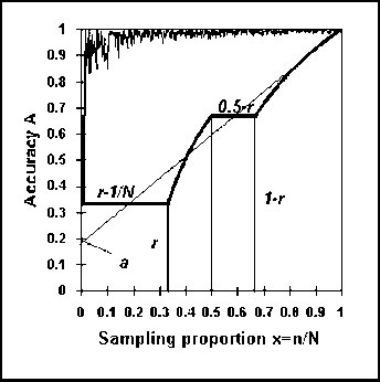
Figure 5.3 illustrates the formulation of the global line G(x) with an area equal to that formed by the mixed W(x) curve.

Fig. 5.3. The mixed W(x) curve and its equivalent global line G(x)

5.4 Formulae summarizing the global boundaries G(x)

Based on the conclusions of the earlier sections and the formulae (5.1), (5.5), (5.6) and (5.18), it is evident that the construction of a global boundary line of the form:

is a direct function of the WOMA value which, in turn, is based on the assumption as to whether a target population of size N may or may not be concave. Thus the value of the primary parameter in the formulation of G(x) is given by:

Population can be concave

Population cannot be concave

The parameter a representing the intercept of G(x) with the A-axis is given by the single formula:

For large populations the intercept a takes the limit value of 0.189 (concave populations) or 0.5 (non-concave populations).