The A-curves examined so far have permitted an understanding of the growth pattern of the accuracy A and were the basis for formulating feasible domains for all types of hyperbolic A-curves in populations of a given size N. However, with N increasing, the relationship between A and the independent variable x defined in (3.1) has the following two undesirable properties:
(a) The global boundaries G(x) of the feasible domains remain fixed and show no correlation to the top-left movement of the majority of A-curves that are expected to have a hyperbolic-type shape.
(b) The segments of the curves corresponding to small or moderate sample proportions are too close to the A-axis and do not provide a clear view of the accuracy growth in these operationally important regions.
The above observations point to the need of finding a new relationship between A and sample size.
In the discussed "hyperbolic-type" A-curves the
independent variable  takes
values between
  and 1 and
most of the A-curves are expected to follow a "hyperbolic-type" pattern.
This pattern is of the general form:
|
|
(6.1) |
where the two parameters c and k are subject to:
 and
and
 .
.
When  the
curve A(x) takes the minimum value:

while for x=1 it becomes 1.
Since the sample size n can always be expressed as
 , it follows that expression
(6.1) can be written as:
|
|
or: |
|
|
(6.2) |
where the new independent variable x is given by:
|
|
(6.3) |
In this manner the "hyperbolic-type" curves have been transformed to an exponential function in a new system of coordinates where the independent variable x is now defined as in (6.3).
The new variable x varies between 0 (when n=1)
and 1 (when n=N). The mid value x=0.5 corresponds to
 .
.
Concerning the boundary lines given by:
 with
with

these take now the form:
|
|
|
|
|
(6.4) |
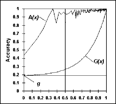
Figure 6.1 illustrates an example of an exponential A-curve and the transformed boundary line G(x) using the relationship between A and the new independent variable x.
Fig. 6.1. Transformed A-curve and boundary G(x) when x=logn/logN

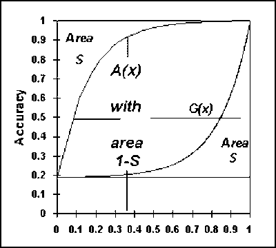
Fig. 6.2. The area S formed by the exponential boundary G(x)

We will now prove that the critical sample size is when x=0.5 and that it is at that value of x that the exponential A-curves reach a breakpoint and start a steady and slow growth versus 1.
We start with the observation that for each A(x) defined as in (6.2) there exists an associate curve B(x) of the form:
|
|
(6.5) |
For x=0 the A(x) and B(x) curves take the
same value  while for
x=1 they both become 1.
However, the two curves follow contrary patterns of growth. The A-curve has a rapid growth up to a certain value of x and from then on it grows steadily until it becomes 1. The curve B shows a slow and steady growth for small values of x and beyond a certain value of x it starts a rapid growth until it also becomes 1.
Evidently the critical value of x is at a point where the difference A(x)-B(x) becomes maximum as it is from that point on that the growth of A becomes slower and steadier and that of B faster.
In terms of differential calculus we are seeking a critical point x at which the first derivatives of both A(x) and B(x) have the same value, that is when:

or when -x=x-1 which is equivalent to x=0.5.
It has thus been shown that the breakpoint in the exponential
accuracy growth corresponds to x=0.5, equivalent to sample size
 .
.
In the previous Section it was shown that all A-curves that follow an exponential pattern reach a breakpoint at a critical sample size corresponding to x=0.5. Thus an advantageous feature of the exponential A-curves is that they magnify the growth pattern of A in the operationally important regions where the sample size is small or moderate.
As the population size N increases the exponential A-curves tend to move to the upper left part of the plot while the now exponential boundary curves move in opposite direction. Moreover, the area between the exponential boundary and the horizontal line starting from its intercept with the A-axis, tends to become smaller with a limit value of zero.
We will now introduce two additional secondary parameters that both are functions of the parameter a. The first parameter, denoted by g, is where the exponential boundary G(x) intersects the A-axis. Using expression (6.4) we obtain:
|
|
(6.6) |
The second parameter, denoted by S, represents the area formed by the exponential boundary G(x) and the horizontal line starting from g. In the next section it will be shown that this area is given by:
|
|
(6.7) |
A last observation concerns the breakpoints of the A-curves which, as already discussed, are always to be found on the vertical line x=0.5. As N increases these points move upwards with their distance from the horizontal line A=1 following a decreasing pattern and, as it will be seen in the coming sections, always staying above the point whose distance from the x-axis is equal to 1-S.
In this section we will explain the derivation of the parameter S used in expression (6.7). This parameter expresses the area formed between the exponential boundary G(x), defined in (6.4), and the horizontal line starting from its intercept g with the A-axis as given by (6.6).
Since the area below the horizontal line A=g is also g, the area S will be computed by first integrating G(x) in the interval [0, 1] and then subtracting g.
We can thus write:

from which we obtain:

hence expression (6.7).
A concluding observation regarding the parameter S is that the area formed by the accuracy curve of the family (6.2) with parameters c=a and k=1:
|
|
(6.8) |
is equal to 1-S, as shown in Figure 6.2. This is easily
verified by evaluating the integral
 and taking into account
expression (6.7):
|
|
|
|
|
|
|
|
|
|
|
(6.9) |