7. GEOMETRICAL LIMITS FOR EXPONENTIAL ACCURACY CURVES

7.1 A fundamental property of exponential A-curves

A physical property of the family of exponential accuracy curves defined in (6.2), is that they start from a point higher than the pessimistic intercept (=lowest accuracy at sample size 1) and form an area larger than that defined by the curve:

which starts from g.

This property has not been proved mathematically but it is based on repeated experiments, it therefore constitutes the third major assumption of the present study (see also introductory Section). In descriptive terms it can be explained by considering that the differences of the areas beyond the point x=0.5 are negligible since all curves start to converge steadily towards 1, while to the left of x=0.5 the differences are much more significant since most curves of the family (6.2) will tend to start from a point always higher than g.

The area formed by the curve (7.1) has already been computed in Section 6.4 and proved to be equal to 1-S, with S defined as in (6.7).

It is thus expected that for a population with size N the family of exponential curves:

will start from a point higher than and form an area greater than 1-S. Consequently any straight line of the type:

and forming an area equal to that of (7.1a) will intersect the vertical axis x=0.5 at a point lower than the one formed by the curve (7.1a).

We now consider a "pessimistic" hypothetical line of the form (7.2) forming an area equal to 1-S, in which case the intercept h will be:

and the "pessimistic" line (7.2) can thus be expressed as:

7.2 Intersection of exponential A-curves with the x=0.5 axis

The pessimistic hypothetical line A(x) defined in (7.4) intersects the vertical axis x=0.5 at a point:

and all the other lines with areas equal to that of (7.1a) will be intersecting the vertical axis x=0.5 at a point higher than 1-S. It can thus be concluded that the exponential A-curves of the type (7.1a) will also intersect the vertical line x=0.5 at a point higher than 1-S.

7.3 Construction of a lower limit curve A_(x)

Based on the observations made in the previous section and using the intercept a defined in (5.22) together with its two derivatives g and S given in (6.6) and (6.7), it is now possible to formulate a feasible domain exclusively for the expected exponential accuracy curves. Such a domain should be expected to also have an exponential boundary enveloping most of the expected A-curves.

The general form of an exponential boundary, denoted by , should not be a member of the family (7.1a) but an "artificial" curve defined as:

and forced to pass through the points g, 1-S and 1. Its three parameters are subject to the following three conditions:

(a) For x=0 its intercept with the A-axis must be equal to g:

(b) Its intercept with the vertical line x=0.5 must be 1-S:

For x=1 it must take the value 1:

By subtracting (7.6) from (7.7) and (7.7) from (7.8) we obtain:

By dividing (7.10) by (7.9) and solving for k we obtain:

By substituting k in (7.9) and using (7.6) we find:

To be noted that the parameters g and S used in the formulation of the limit curve defined in (7.5) are only a function of the intercept a which, by referring to expressions (5.20) and (5.21) for the primary parameter , is only a function of the population size N.

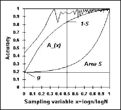
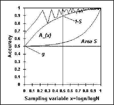
Figures 7.1 and 7.2 illustrate the geometrical model described above for two populations with size N=100. In the first case no assumption could be made as to the distribution of the population and the geometric limits made use of expressions (5.20) and (5.22) for the computation of parameter a. In the second case it was assumed that the population cannot be concave, and a was computed using expressions (5.21) and (5.22), thus resulting in less pessimistic limits for the domain of exponential A-curves.

Fig. 7.1. Feasible exponential curves for possibly concave populations (N=100)

Fig. 7.2. Feasible exponential curves for non concave populations (N=100)