![]()
![]()
![]()
7.1 Trawl selection
7.2 Recruitment
7.3 Size limits
7.4 Gill-net selection
7.5 Exercises
Not all sizes or ages of fish undergo the same fishing mortality: small fishes may escape through the meshes of a net, or not be in the main fished area. It is useful to distinguish the part due purely to behaviour (in the widest sense) of the fish themselves - recruitment - and that due to the properties of the gear selection.
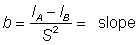
Selection is simplest in the bag-type of gear - trawls, seines, etc. For these gears it is usual to assume that the size composition of the fish entering the mouth of the net is the same as that in the immediate vicinity of the gear. The selectivity of such gears therefore becomes a question of escape, through the meshes, of fish which have entered the net. For many species there is evidence to show that most of this escape occurs through the cod-end. Selectivity can therefore be determined directly if the numbers of each size of fish entering the net can be estimated, either by attaching a small-meshed cover over the cod-end or other parts, or from the size-composition of the catches of nets of much smaller meshes fished at the same time and place. Whichever method is used, the results can be expressed as the proportion of fish at each length entering the net which are retained in the cod-end. When these proportions are plotted against length, the selection curve of the net for the species concerned is obtained. A typical example is shown in Figure 7.1.
FIGURE 7.1. - Simple selection curve. Determination of mean selection length.
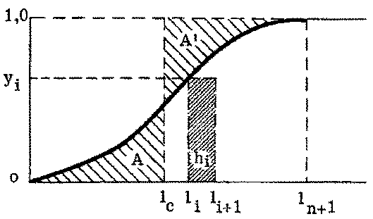
A selection curve may extend over a range of length of fish of perhaps 10 cm or more, which means that as young fish begin to grow into the selection range they at first suffer only a low fishing mortality. As they grow larger, their chance of escaping from the net (having entered it) gets less, until, eventually, they are too large to escape at all; only then are they exposed to the full fishing mortality rate - whatever that may be. Although it is possible to introduce this progressive change of fishing mortality coefficient over the selection range into yield assessments, it is usually sufficient to represent the selection process by a single mean selection length lc, and assume that all fish of length less than lc are released, and that all those greater than lc are retained by the gear, and experience the full fishing mortality.
The important quantity is therefore
|
tc |
= mean selection age |
|
|
= mean age of entry to the catch, or mean age at first capture |
In Figure 7.1 the mean selection length lc is the length which makes the two shaded areas A and A' equal. If the selection curve is symmetrical, or nearly so, this will be the length at the midpoint of the curve, i.e. the 50 percent length, at which half the fish entering the net escape and half are retained. If the curve is not symmetrical, lc can be calculated by equating the two areas between the selection curve and the y-axis, and between the line l = lc, and the y-axis. Suppose the lengths are classified, the ith class being of size hi and limited by the lengths li, and li+1; the corresponding ordinate to the ith class is yi where i = 0, 1, 2, ... n.
Then the area to the left of the selection curve is equal to the area of the rectangle of height 1 and base ln+1 minus the area under the selection curve. This last area can be approximated by the sum of the rectangle areas for each length-class, i.e., S hi·yi. The total area to the left of the selection curve is therefore ln+1 - S hi·yi, which, as the total height of the curve is 1, will equal lc. If hi is constant and equal to 1 cm, lc = ln+1 - S yi.
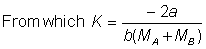
For trawls, the mean selection length lc is generally proportional to the mesh size, m, i.e.
lc == b · m
where b is the selection factor
This expression enables the mean selection factor for any mesh size to be estimated from the results of experiments with a small number of different mesh sizes. The selection factor also does not vary much for fish of roughly the same shape. There is some variation in selection factor with the condition of the fish, and also with the material and construction of the meshes; light flexible materials (e.g. nylon) give higher selection factors than thicker materials (e.g. manila).
Besides the mean selection length (50 percent point) selection curves also differ in their sharpness - whether selection occurs over a small or wide range of sizes. This is usually measured by the selection range - the difference between the lengths at which 25 percent and 75 percent of the fish are retained by the gear.
Recruitment is the process in which young fish enter the exploited area and become liable to contact with the fishing gear. This may involve an actual movement, as in the North sea plaice, which moves, when relatively old (about three to four years), from the shallow nursery area along the coast into the main fishing grounds. Recruitment may involve only a change in habit, such as in the North sea haddock, where young and old occur in the same areas, with the very young fish being pelagic, and recruiting to the exploited phase when they take up a demersal habitat in the autumn of their first year of life. Mathematically, the important quantity is tr = mean age at recruitment.
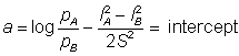
Recruitment is, by its nature, much less easy to express in quantitative terms than mesh selection. As the main interest is in the combined effect of recruitment and selection - i.e. the pattern of entry into the catch - the recruitment pattern is very important when it is above, or overlaps, the range of gear selection, but not when it is complete before gear selection starts. If therefore all fish have been recruited at a size below the selection range of any likely mesh size, then the precise pattern of recruitment may be ignored, and it can be taken arbitrarily as occurring at some convenient length or age below the selection range (see Figure 7.1). Where important, the general form of the recruitment curve may be determined by a proper knowledge of the biology of the species, and possibly estimated with greater accuracy by surveys, with research vessels, of the young fish both on and off the main fishing grounds. Failing this an estimate may be obtained by comparing the size composition of actual catches of commercial vessels with the known selectivity of the gear in use. Normally the recruitment will occur over a range of sizes and may be described by the same type of curve as the selection curve of Figure 7.1.
If selection and recruitment are occurring over the same range, as in Figure 7.2, then the effective selection, i.e. the proportion Pl of the full fishing mortality to which the fish of a given size in the stock are exposed will be given by the equation
Pl = rl × Sl........................................... (7.1)
where
rl == proportion recruited, i.e. ordinate of recruitment curve,
Sl = proportion of those entering the net which are retained, i.e. the ordinate of the selection curve.
FIGURE 7.2. - Combination of a selection curve and recruitment. Recruitment over a spread of lengths.
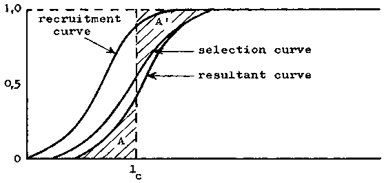
Thus the resultant selection curve, which expresses the effective entry of fish to the catch, is obtained as the product of the recruitment and mesh selection curves, and from it the resultant mean selection length can be determined as before by equating the two areas A, A'.
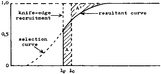
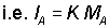
Sometimes, as in cases where the recruits migrate into a fishing area, recruitment, in terms of length, can be quite sharp, approaching in the extreme case knife-edge selection at a threshold length lr, as in Figure 7.3. Fish below length lr, suffer no fishing mortality at all, since they are not within the range of the gear. But on reaching length lr, they are at once exposed to a high fishing mortality (as drawn in Figure 7.3 more than half of the full fishing mortality). The resultant selection curve in this case therefore starts at length lr, and rises vertically to the selection curve of the gear; thereafter it is identical with the selection curve itself. Again, however, the mean selection length lc can be calculated from this resultant curve, in this case lc is such that the two areas A and A' of Figure 7.3 are equal.
FIGURE 7.3. - Knife-edge recruitment.
If a minimum legal size limit, ls say, is set within or above the selection range of the gear in use, the entry to the landed catch can be represented by a curve which starts at ls, and rises vertically until the true selection curve is reached (see Figure 7.4). The mean selection length lc is calculated in a similar way and is such as to equalize the areas A and A' of Figure 7.4.
FIGURE 7.4. - Effect of size limit (ls) on the effective selection curve.
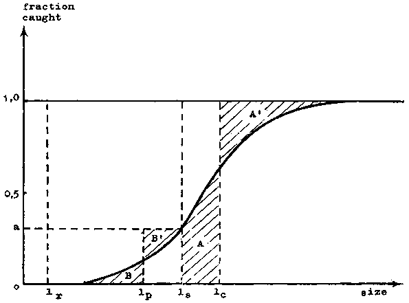
Undersized fish will also be taken, and since they cannot be landed they must be rejected at sea. The effect of this capture and rejection on the yield from the stock depends on how many of the rejected fish survive. If all survive, the situation is the same as if the recruitment curve to the landed catch were the true selection curve.
If on the other hand, some or all undersized fish die after rejection, each year-class is subjected to a certain fishing mortality before it reaches length ls, as represented by the lower part of the selection curve in Figure 7.4. The resultant fishing mortality coefficient which takes account of the capture and rejection of undersized fish is obtained by calculating the mean of that part of the selection curve which is below the size limit. Calling this mean length lp, then it is such as to equalize the areas B and B' of Figure 7.4. In other words, it is assumed that fish are not caught at all until they reach length lp, and are then subjected to the constant fraction a of the full fishing mortality rate until they reach size ls (a is the ordinate at length ls, see Figure 7.4). If growth from length lp to length ls occupies a period ts - tp (see below) and the fraction q of rejected fish die, then the year-class is reduced by the factor
....................... (7.2)
as a result of capture and rejection of undersized fish before it enters the marketable size range. In this expression F is the full fishing coefficient to which fish are exposed when they have grown beyond the selection range of the gear.
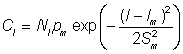
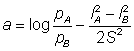
The selectivity of gill-nets is such that the proportion of fish retained is a maximum at some optimum size, and falls off for fish bigger or smaller than this optimum. If the size distribution of the fish in the fishing area can be determined directly by using some gear which is nearly unselective, or where selectivity is known, e.g. a trawl, then the selectivity of the gill-net may be determined at once. That is, if the numbers of a given size, l, of fish caught per unit fishing time by gill-nets and the presumed nonselective gear are GCl, TCl respectively, the fishing mortality exerted by the gill-net on fish of length/will be proportional to
When a nonselective gear cannot easily be used, then the selective properties are best estimated by using a range of gill-nets of several different sizes. For any particular size of fish the distribution of catches by different mesh sizes will be analogous to the distribution of catches by a particular mesh size of different sizes of fish, having a maximum at some optimum mesh size, and falling off at each side. From the data of catches by different nets (adjusted if necessary to allow for different total fishing time by different mesh sizes) such distributions can be obtained for each size of fish. These can be combined by expressing both variables in standard terms - mesh size as the ratio of its perimeter to the girth of the given size of fish, or as a ratio of its size to the most efficient mesh size for that size of fish, and numbers of fish caught as a ratio of the numbers caught with the mesh used and with the most efficient mesh (see McCombie and Fry, 1960; Gulland and Harding, 1961).
If it is assumed that each mesh has the same optimum fishing power, i.e. causes the same fishing mortality on the size of fish for which it is most efficient, then the combined data can be used at once to give not only the relative efficiencies of different nets on a given size of fish, but for a net of a given mesh size, the relative efficiencies on different sizes of fish, i.e. its selectivity.
The selectivity may also be estimated by comparing catches of only two mesh sizes, provided some assumption is made concerning the form of the selection curve. This is often close to normal, and if it is assumed in fact to be normal, then putting
Cl = catch of fish of length l per unit fishing time
where
Nl = number of fish of length l liable to capture by the gear
pm = fishing power of net of mesh size m
lm = length of fish for which the mesh size m is most efficient
Sm = standard deviation of the mesh selection curve
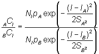
If two meshes, A and B, are fished on the same population, then, in the obvious notation
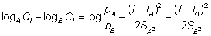
or, taking logarithms to base e,
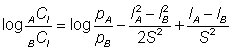
and, if it is further assumed that the standard derivation of the selection curve is constant, i.e. SA = SB = S, this reduces to
The right-hand side is linear in l, that is, can be expressed in the standard form a + bl, where
Thus if the log of ratio of the catches per unit time of nets of different size are plotted against length the result is a straight line, from which can be estimated
From this lA, lB and S2 cannot be estimated separately, and hence the selection curves determined, without some extra assumptions; however it is reasonable to assume (as in the previous section for a range of mesh sizes) that the fishing powers of the two nets are equal, and also that the optimum length is proportional to mesh size (usually in practice equivalent to a fish whose girth is slightly greater than, say 1.1 times, the perimeter of the mesh).
and hence the selection curves can be determined.
Other assumptions can be made about the shape of the selection curve; in particular it might be assumed as above that the curve is normal, but that the standard deviation is proportional to the mesh size. This model often fits the observed data better than the model based on constant standard deviation (see Regier and Robson [1966] for a full review of gill-net selectivity).
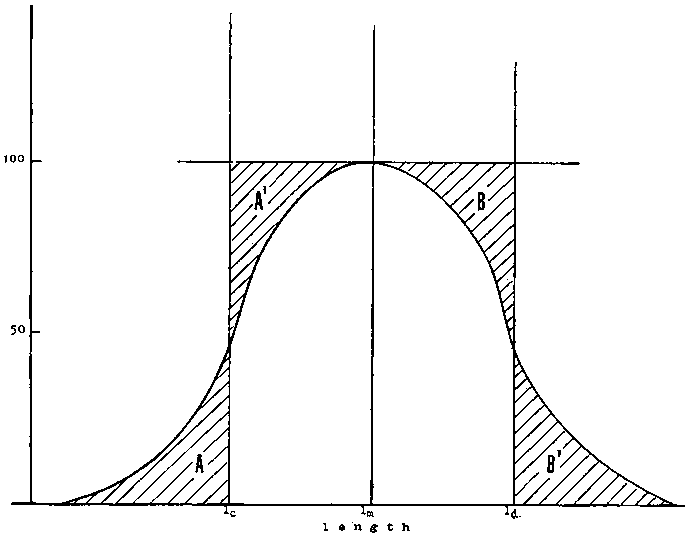
When the selection curve of the gill-net has been determined, subsequent population analysis is simpler if the curve can be represented by a more simple form, analogous to the knife-edge approximation to the trawl selection. Two selection lengths are needed, 4, the length at which the fish enter the selection range, and ld, at which they grow out of it. That is, the fishing with a gill-net with the selection curve of Figure 7.5 has the same effect as a constant mortality between lengths lc and ld, where the pairs of shaded areas A and A', and B and B' are equal.
1. (a) Cod-ends of 44 mm and 112 mm fished alternatively gave catches of plaice of equal fishing times as set out in Table 1.
TABLE 1. - PLAICE
|
Length |
44-mm mesh |
112-mm mesh |
|
cm | ||
|
10 |
0 |
0 |
|
11 |
1 |
0 |
|
12 |
2 |
0 |
|
13 |
6 |
0 |
|
14 |
16 |
0 |
|
15 |
18 |
0 |
|
16 |
26 |
0 |
|
17 |
64 |
3 |
|
18 |
121 |
4 |
|
19 |
182 |
10 |
|
20 |
247 |
13 |
|
21 |
292 |
16 |
|
22 |
344 |
37 |
|
23 |
367 |
60 |
|
24 |
355 |
132 |
|
25 |
276 |
190 |
|
26 |
225 |
177 |
|
27 |
147 |
136 |
|
28 |
90 |
97 |
|
29 |
57 |
54 |
|
30 |
26 |
33 |
|
31 |
24 |
26 |
|
32 |
18 |
13 |
|
33 |
10 |
9 |
|
34 |
12 |
7 |
|
35 |
5 |
6 |
|
36 |
10 |
5 |
|
37 |
6 |
2 |
|
38 |
3 |
4 |
|
39 |
2 |
2 |
|
40 |
2 |
3 |
|
41 |
0 |
1 |
|
42 |
0 |
2 |
|
43 |
0 |
2 |
|
44 |
0 |
1 |
|
45 |
0 |
1 |
|
46 |
0 |
1 |
|
47 |
0 |
0 |
|
48 |
0 |
0 |
TABLE 2. - WRITING
|
Length |
Cod-end |
Cover |
|
cm | ||
|
10 |
0 |
0 |
|
11 |
0 |
0 |
|
12 |
0 |
3 |
|
13 |
0 |
7 |
|
14 |
0 |
21 |
|
15 |
0 |
27 |
|
16 |
0 |
23 |
|
17 |
0 |
19 |
|
18 |
2 |
20 |
|
19 |
3 |
83 |
|
20 |
23 |
219 |
|
21 |
68 |
302 |
|
22 |
89 |
256 |
|
23 |
79 |
154 |
|
24 |
115 |
55 |
|
25 |
106 |
42 |
|
26 |
87 |
18 |
|
27 |
63 |
7 |
|
28 |
55 |
0 |
|
29 |
38 |
2 |
|
30 |
34 |
0 |
|
31 |
11 |
0 |
|
32 |
11 |
0 |
|
33 |
6 |
0 |
|
34 |
9 |
0 |
|
35 |
5 |
0 |
|
36 |
2 |
0 |
|
37 |
1 |
0 |
|
38 |
1 |
0 |
|
39 |
0 |
0 |
(b) A cod-end of 74 mm fitted with a small-meshed cover gave catches of whiting distributed between the cod-end and cover as in Table 2.
Draw the selection curves for plaice and whiting from these data and determine the mean selection lengths (lc). Note that the number entering the net is for (a) (alternate hauls) equal to the catch in the small-meshed net, but for (b) is the sum of the fish retained in the cod-end, and those which went through the meshes, i.e. in the cover.
Calculate selection factors.
2. An approximate recruitment curve for the United Kingdom North sea plaice fishery is as follows:
|
Length (cm) |
20 |
21 |
22 |
23 |
24 |
25 |
26 |
27 |
28 |
29 |
30 |
31 |
32 |
33 |
34 |
|
Fraction recruited... |
0.02 |
0.05 |
0.08 |
0.16 |
0.27 |
0.38 |
0.48 |
0.62 |
0.75 |
0.86 |
0.94 |
0.97 |
0.99 |
1.00 |
1.00 |
Calculate the resultant selection curve with a mesh of 112 mm (using the result from Exercise 1) and hence the value of 4.
If instead of the above recruitment curve, recruitment was found to be effectively "knife-edge" at 26 cm, what would be the value of lc with a 112-mm mesh?
3. Convert the above estimate of lc for plaice and whiting to age (tc) using the von Bertalanffy equation and parameter values as follows:
|
|
K =0.095 |
|
K= 0.32 |
|
Plaice |
L¥ = 68 cm |
Whiting |
L¥ = 45.5 cm |
|
|
t0 = - 0.8 year |
|
t0 = - 0.4 year |
4. The percentage length-distributions of cod caught by gill-nets and purse-seines at Lofoten in 1952 were as follows (data from Rollefsen, 1952)
|
Length (cm) |
65- |
70- |
75- |
80- |
85- |
90- |
95- |
100- |
105- |
110- |
115- |
120+ |
|
Purse-seine ..... |
2 |
4 |
8 |
13 |
20 |
28 |
35 |
34 |
25 |
15 |
8 |
5 |
|
Gill-nets .......... |
0 |
2 |
5 |
15 |
30 |
50 |
45 |
27 |
15 |
5 |
2 |
1 |
Assuming there is no selection by purse-seines, determine the form of the selection curve of the gill-nets. What size of fish is caught most efficiently by gill-nets?
5. Nine sizes of gill-net were used for catching salmon in the Frazer river in 1947 and 1948. The numbers of fish of sizes caught by each mesh (adjusted for different fishing times) were as follows (data adapted from Peterson, 1954)
|
Fork length
|
Mesh sizes |
||||||||
|
cm |
|||||||||
|
13.5 |
14.0 |
14.8 |
15.4 |
15.9 |
16.6 |
17.8 |
19.0 |
20.6 |
|
|
50-51 |
6 |
4 |
|
|
|
|
|
|
|
|
52-53 |
52 |
11 |
1 |
1 |
- |
- |
- |
- |
- |
|
54-55 |
102 |
91 |
16 |
4 |
4 |
2 |
- |
2 |
2 |
|
56-57 |
295 |
232 |
131 |
61 |
17 |
13 |
3 |
1 |
2 |
|
58-59 |
309 |
318 |
362 |
243 |
95 |
26 |
4 |
2 |
1 |
|
60-61 |
118 |
173 |
326 |
342 |
199 |
100 |
10 |
8 |
1 |
|
62-63 |
79 |
87 |
191 |
239 |
202 |
201 |
39 |
10 |
6 |
|
64-65 |
27 |
48 |
111 |
143 |
133 |
185 |
72 |
16 |
3 |
|
66-67 |
14 |
17 |
44 |
51 |
52 |
122 |
74 |
27 |
3 |
|
68-69 |
8 |
6 |
14 |
23 |
25 |
59 |
65 |
51 |
1 |
|
70-71 |
7 |
3 |
8 |
14 |
15 |
16 |
34 |
22 |
2 |
|
72-73 |
|
3 |
1 |
2 |
5 |
4 |
6 |
10 |
1 |
|
74-75 |
|
|
|
|
|
|
|
1 |
|
(a) Graphical method. By plotting for each size group separately the numbers caught against mesh size, estimate the numbers of each size of fish which would be caught by the most efficient mesh for that size of fish. Hence express the catch of any mesh as a percentage of the potential catch by the most efficient mesh, i.e. the selectivity of that mesh size for that size of fish.
Combine these selection curves for all meshes by expressing the mesh size as a proportion of the most effective mesh for the length group in question. Hence obtain a single combined selection curve of a gill-net on salmon.
(V) Analytic method. Calculate the logarithm of the ratio of catches of fish of a given size taken by pairs of adjacent mesh sizes. Assuming the selection curve for each mesh is normal and of constant variance, and that the mean selection length of any mesh is proportional to the mesh size, calculate the selection curve for each mesh.
![]()
![]()
![]()


