![]()
![]()
![]()
10.1 INTRODUCTION
10.2 SINGLE COHORT
10.3 MULTIPLE COHORTS
10.4 STRUCTURED LINK MODELS
10.5 CROSSLINKED MODELS
10.6 BOOTSTRAPPING BASED ON MONTE CARLO SIMULATIONS
Simulated data is used for these examples. This has the advantage that the true parameters and models that produce the data are known. Hence, any structural errors in the assessments are known and data is recorded with complete accuracy. All errors stem from observation errors, which are log-normal and relatively large, however.
By introducing new data and models, we show how increasingly complex, but more realistic models can be fitted to fisheries data. We start by considering models of single cohorts, where many of the basic modelling techniques are introduced. Cross-cohort models are then discussed mainly as separable VPA. We then consider generalised linear models as structured link models and how ANOVA techniques may be used to study the structure in complex models and some use of weights in allowing different data sets to be linked to the same parameters. Finally, we show how Monte Carlo simulation techniques can be used to assess the uncertainty of the results.
The examples are developed for Microsoft Excel, using Visual Basic for Applications and the add-in optimiser, Solver. Other spreadsheet software could equally well be used.
10.2.1 No Abundance Index
10.2.2 One Abundance Index
10.2.3 Uncertain Catch
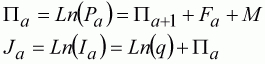
The cohort model is based on the principle that if we know how many fish died from natural causes and we know how many were caught, we can reconstruct the history of the cohort (Table 10.1).
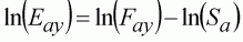
We need to give the final population size (or terminal F) for backward calculation, or recruitment (or initial F) for forward calculation. In this case, the Newton-Raphson method was used, but for variety, in the forward calculation form (see Macro 10.1). The recruitment and age-dependent natural mortality were provided as the input parameters. The population is modelled loosely on temperate water groundfish. The natural mortality figures are thought to represent reasonable levels for these species. It is often assumed that younger fish have higher mortality rates due to their smaller size, making them more vulnerable to predation.
Given the recruitment, we solve the Baranov equation (see Section 4.7 Solving the VPA Equations) to obtain the next population size, and so on down the cohort ages to the last year or age as a appropriate. The fishing mortality, Fa, is calculated as:
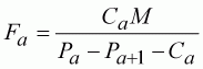 (109)
(109)
Table 10.1 Cohort catches (Ca), natural mortality (M), population size (Pa) and fishing mortality (Fa) calculated from the catch data and recruitment (population age 1). The plus-group “11+” FA is not calculated because it depends on contributions from other cohorts. This will be dealt with later (Section 10.3), and this age group can be ignored for now.
|
Age |
Ca |
M |
Population |
Fa |
|
1 |
37937 |
0.80 |
560282 |
0.103 |
|
2 |
25608 |
0.35 |
227153 |
0.143 |
|
3 |
27537 |
0.25 |
138773 |
0.252 |
|
4 |
19460 |
0.20 |
83965 |
0.294 |
|
5 |
12784 |
0.20 |
51252 |
0.320 |
|
6 |
11391 |
0.20 |
30475 |
0.526 |
|
7 |
5618 |
0.20 |
14750 |
0.539 |
|
8 |
2641 |
0.20 |
7046 |
0.527 |
|
9 |
1253 |
0.20 |
3404 |
0.515 |
|
10 |
647 |
0.20 |
1665 |
0.553 |
|
11+ |
726 |
0.20 |
785 |
|
|
Function SolFVPANR(M, Ca, Na As Double) As Double |
||
|
Dim fx, dfx, Na_1, DeltaNa, Z As Double |
||
|
|
‘Estimate initial Nt+1 from Pope’s cohort
equation |
|
|
|
|
|
|
Na_1 = Na * Exp(-M) |
‘Calculate Na+1 with no fishing |
|
|
DeltaNa = -Ca * Exp(-M / 2) |
‘Calculate equivalent deaths due to fishing |
|
|
|
|
|
|
Do While Abs(DeltaNa) > 0.1 |
‘Test current accuracy |
|
|
|
Na_1 = Na_1 + DeltaNa |
‘Add correction to N t+1 |
|
|
Z = Log(Na) - Log(Na_1) |
‘Calculate total mortality |
|
|
fx = (1 - M / Z) * (Na - Na_1) - Ca |
‘Calculate the function |
|
|
dfx = -1 + (Z - (Na - Na_1) / Na_1) * M / (Z * Z) |
‘And its derivative |
|
|
DeltaNa = -fx / dfx |
‘Calculate the new correction factor |
|
|
|
|
|
Loop |
|
|
|
SolFVPANR = Na_1 |
‘Return solution |
|
|
End Function |
|
|
In this case, the recruitment, M and all catches are known from the simulation. By using these values, we are simply repeating the simulation backwards, so the result is exact. Of course, in practice we would not know the recruitment or natural mortality exactly. In these examples, we will not be concerned with estimating natural mortality, but we will look in detail at the problem of estimating recruitment. It is worth remembering that the resulting view given by the examples will be optimistic. In practice natural mortality is never known, and may well vary with time and age.
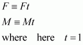
One final point, which also applies to all further examples as well, is the implicit time unit in the mortality rates. If the time units vary, we simply multiply the rates by the new time unit in the model. Hence for all the references to F and M in the models below could be expanded to allow different time periods, as:
 (110)
(110)
In cases where the final population size in the last age group is unknown, we need to estimate it. In many cases, there is additional data besides catches, which can be used as an abundance index. Here we introduce some additional data representing a scientific survey carried out in the third quarter of each year.
The timing of the index is critical where there is a significant change of population size within the season. Even if there is not thought to be a big change in population size, this is a simple adjustment to make and therefore it should not be neglected. For this simulated survey, the population must be adjusted to the number in July-September, approximately the point in time when the survey was conducted.
The population model is fitted by minimising the squared difference between the observed and expected index, the expected index being based on the population model. We therefore need to develop a link model, which will allow the expected index to be calculated from the population model. Because this is a scientific survey, it is assumed that the sampling design will ensure the index will be proportional to the population size.
We estimate the mean of the abundance index for each parameter as:
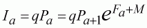 (111)
(111)
To fit the model, we need to be able to calculate the differential equations with respect to each of the parameters, so that we can calculate the covariance (inverse Hessian) matrix on each iteration. The first point we can note is that, as the population size is proportional to the index, the slope is equal to the population size, so:
 (112)
(112)
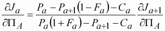
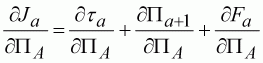
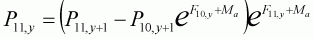
The analysis is a little more complicated for the other parameter, the terminal population size (PA). In this case, we can only define the partial differential with respect to future populations, moving towards the terminal population. Noting that Fa, unlike catches and natural mortality, depends on the population estimates (Equation 109), we find:
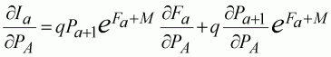 (113)
(113)
From Equation 109, we can define the differential with respect to Fa as:
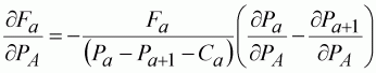 (114)
(114)
By substituting Equation 114 into Equation 113 and rearranging, we find the recursive differential equation:
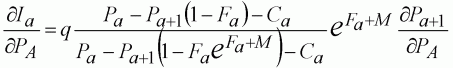 (115)
(115)
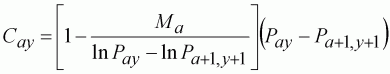
The least-squares partial differentials with respect to each of the parameters is given by:
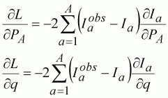 (116)
(116)
where Iaobs is the observed index value.
We can calculate the value for each differential equation at each age, and therefore define the approximation of the least-squares (approximate) Hessian matrix as:
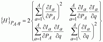 (117)
(117)
The inverse of this matrix is the covariance matrix, and can be used in the non-linear fitting process. We are now ready to apply the Newton-Raphson method, using the Hessian matrix to move towards the minimum point, where the partial differentials (Equation 116) are zero. The scheme here is:
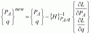 (118)
(118)
The table containing the calculations for Equation 118 can be set up in a spreadsheet (Table 10.2).
Table 10.2 Final results of the table fitting the VPA population model to the observed abundance index. The error is the difference between the observed index and the index estimated from the model (i.e. Iaobs-Ia). Notice, the differential dIa/dq is identical to the population size, Pa. As in the previous analysis, the 11+ group is ignored as it contains animals from other cohorts not modelled here.
|
Linear Index |
|
|
|
PA |
4624.22 |
|
|
|
||
|
|
|
|
|
|
q |
1.03 10-5 |
|
|
|
|
|
Age |
Ca |
Iaobs |
M |
Pa |
Fa |
Ia |
Error |
(Error)2 |
dIa/dPA |
dIa/dq |
|
1 |
37937 |
6.3974 |
0.80 |
600773 |
0.096 |
6.187 |
0.211 |
0.044 |
13.622 |
6.008 105 |
|
2 |
25608 |
1.7395 |
0.35 |
245336 |
0.132 |
2.526 |
-0.787 |
0.619 |
6.117 |
2.453 105 |
|
3 |
27537 |
1.6226 |
0.25 |
151579 |
0.229 |
1.561 |
0.062 |
0.004 |
4.308 |
1.516 105 |
|
4 |
19460 |
1.7253 |
0.20 |
93927 |
0.258 |
0.967 |
0.758 |
0.575 |
3.352 |
9.393 104 |
|
5 |
12784 |
0.4771 |
0.20 |
59398 |
0.270 |
0.612 |
-0.135 |
0.018 |
2.741 |
5.940 104 |
|
6 |
11391 |
0.2721 |
0.20 |
37134 |
0.410 |
0.382 |
-0.110 |
0.012 |
2.242 |
3.713 104 |
|
7 |
5618 |
0.1729 |
0.20 |
20183 |
0.364 |
0.208 |
-0.035 |
0.001 |
1.830 |
2.018 104 |
|
8 |
2641 |
0.0559 |
0.20 |
11480 |
0.291 |
0.118 |
-0.062 |
0.004 |
1.495 |
1.148 104 |
|
9 |
1253 |
0.0255 |
0.20 |
7025 |
0.218 |
0.072 |
-0.047 |
0.002 |
1.222 |
7.025 103 |
|
10 |
647 |
0.0173 |
0.20 |
4624 |
0.033 |
0.048 |
-0.030 |
0.001 |
1.000 |
4.624 103 |
|
11+ |
726 |
0.0142 |
0.20 |
|
|
|
|
|
|
|
|
|
|
|
|
|
|
|
Sum |
1.281 |
|
|
|
|
|
|
|
|
|
|
df |
8 |
|
|
Table 10.3 The Hessian matrix, its inverse (covariance matrix) and the parameter vectors calculated from Table 10.2. The parameters are taken at their minimum, so the ¶L/¶PA and ¶L/¶q differentials are relatively close to zero (with respect to their variances). The Net Change from multiplying the differential by the covariance matrix is very small, indicating convergence. Hence the New PA and q do not change significantly from those in Table 10.2. Note that the correlation between the parameters is very high, so an estimate for either of the parameters will be accurate only if the other parameter is known.
|
Hessian Matrix |
PA |
q |
|
PA |
546.7635 |
21931023.2 |
|
q |
21931023 |
9.169 10+11 |
|
Covariance Matrix |
PA |
q |
|
PA |
0.04507753 |
-1.0782 10-06 |
|
q |
-1.0782 10-06 |
2.6881 10-11 |
|
Correlation |
-0.980 |
|
|
|
¶L |
Net Change |
|
¶PA |
0.000 |
4.443 10-6 |
|
¶ q |
-4.821 |
-1.115 10-10 |
|
|
New |
|
|
PA |
4624.22 |
|
|
q |
1.03E-05 |
|
The fact that the fitting process behaved poorly should sound some alarm bells. The model may need looking at in more detail. One clear indication is the errors in Table 10.2 are larger for the larger population size. This is strongly indicative of changing variance and skewed errors, which may be corrected by a transformation. We try the same routine, but with a log-transform below.
A log-transform can be undertaken by simply redefining the models in terms of log-values. We now have:
 (119)
(119)
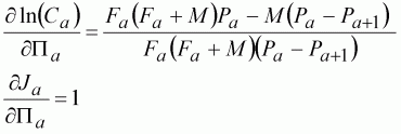
We need to estimate the parameters in their log form, that is the index parameter Ln(q), and the terminal log-population PA. The two partial differentials can be derived through the same process as that described for the linear index:
 (120)
(120)
 (121)
(121)
Otherwise, the method is identical. The calculation Table 10.4 for the fitted model indicates the errors are well behaved, so the largest errors are not associated with the larger populations. Also, the parameter correlation has been much reduced (Table 10.5), so there is less dependency between parameter estimates. The true parameter values known from the simulation suggest that while the q estimate is a little further away from its true value (1.0 10-5), the terminal population size is much closer to the true value of 1665 (from Table 10.1).
Table 10.4 Final results of the table fitting the VPA population model to the observed log abundance index. The error is the difference between the observed log-index and the index estimated from the model (i.e. Jaobs-Ja). The differential dJa/dLn(q) is always equal to 1.0, and therefore not included in this table.
|
Log Model |
|
|
|
|
|
Loge |
|
|
|
|
|
|
|
|
|
|
PA |
1336 |
7.197 |
|
|
|
|
|
|
|
|
|
q |
1.081 10-5 |
-11.435 |
|
|
|
|
Age |
Ca |
Jaobs |
M |
Pa |
Pa |
Fa |
Ja |
Error |
(Error)2 |
dJa/dPA |
|
1 |
37937 |
1.8559 |
0.80 |
555729 |
13.228 |
0.104 |
1.793 |
0.063 |
0.004 |
0.033 |
|
2 |
25608 |
0.5536 |
0.35 |
225109 |
12.324 |
0.144 |
0.889 |
-0.336 |
0.113 |
0.037 |
|
3 |
27537 |
0.4840 |
0.25 |
137333 |
11.830 |
0.255 |
0.395 |
0.089 |
0.008 |
0.043 |
|
4 |
19460 |
0.5454 |
0.20 |
82846 |
11.325 |
0.298 |
-0.110 |
0.656 |
0.430 |
0.055 |
|
5 |
12784 |
-0.7400 |
0.20 |
50337 |
10.826 |
0.327 |
-0.609 |
-0.131 |
0.017 |
0.074 |
|
6 |
11391 |
-1.3017 |
0.20 |
29727 |
10.300 |
0.543 |
-1.135 |
-0.166 |
0.028 |
0.102 |
|
7 |
5618 |
-1.7549 |
0.20 |
14140 |
9.557 |
0.570 |
-1.878 |
0.123 |
0.015 |
0.175 |
|
8 |
2641 |
-2.8845 |
0.20 |
6550 |
8.787 |
0.581 |
-2.648 |
-0.237 |
0.056 |
0.308 |
|
9 |
1253 |
-3.6709 |
0.20 |
3000 |
8.006 |
0.609 |
-3.429 |
-0.242 |
0.059 |
0.547 |
|
10 |
647 |
-4.0569 |
0.20 |
1336 |
7.197 |
0.188 |
-4.238 |
0.181 |
0.033 |
1.000 |
|
11+ |
726 |
-4.2515 |
0.20 |
|
|
|
|
|
|
|
|
|
|
|
|
|
|
|
|
Sum |
0.762 |
|
|
|
|
|
|
|
|
|
|
df |
8 |
|
|
Hessian Matrix |
PA |
Ln(q) |
|
PA |
2.8962 |
4.7479 |
|
Ln(q) |
4.7479 |
20 |
|
Covariance Matrix |
PA |
Ln(q) |
|
PA |
0.5653 |
-0.1342 |
|
Ln(q) |
-0.1342 |
0.08186 |
|
Correlation |
-0.624 |
|
|
|
¶L |
Net Change |
|
¶PA |
0.000 |
3.961 10-7 |
|
¶Ln(q) |
0.000 |
-1.267 10-7 |
|
|
New |
|
|
PA |
7.197 |
|
|
Ln(q) |
-11.435 |
|
Finally, we consider the correction for timing of the observation. This requires that the population size is adjusted to represent the mean population size during the survey.
 (122)
(122)
The proportional decrease in mean population size is derived from integration over the period of the survey:
 (123)
(123)
Again the procedure is exactly the same as that presented above. However, we do need to adjust the partial differential with respect to the terminal population size (dJa/dPA) to account for the within season changes:
 (124)
(124)
 (125)
(125)
A brief perusal of this equation explains why numerical approximations of the differential are popular. The equations become very complicated as models become more realistic. However, the fitting procedure remains the same whether dJa/dPA is estimated numerically or calculated using Equation 125.
Table 10.6 Final results of the table fitting the VPA population model to the observed log abundance index, adjusted for timing of the survey during the season. The differential dJa/dLn(q) is always equal to 1.0, and therefore not included in this table. *Note that in contrast to the previous models, it was not necessary to know the fishing mortality for the final age class (F10). However, to adjust the index for survey timing it is required. In this case, it was assumed to be the same as the fishing mortality in the previous age class (F10= F9), the alternative option being to ignore the final age class’s index (J10).
|
Log Model |
|
|
|
|
Loge |
|
|
|
|
|
|
Index adjusted |
PA |
|
1460 |
7.286 |
|
a |
0.50 |
|
||
|
|
|
|
q |
|
1.316 10-5 |
-11.238 |
|
b |
0.75 |
|
|
Age |
Ca |
Jaobs |
M |
Pa |
Fa |
t |
Ja |
Error |
dPa/dPA |
dJa/dPA |
|
1 |
37937 |
1.3569 |
0.80 |
13.231 |
0.103 |
-0.5625 |
1.431 |
-0.074 |
0.036 |
0.039 |
|
2 |
25608 |
0.3329 |
0.35 |
12.328 |
0.144 |
-0.3079 |
0.782 |
-0.449 |
0.040 |
0.044 |
|
3 |
27537 |
0.3250 |
0.25 |
11.834 |
0.254 |
-0.3145 |
0.282 |
0.043 |
0.046 |
0.055 |
|
4 |
19460 |
0.4153 |
0.20 |
11.330 |
0.296 |
-0.3097 |
-0.218 |
0.633 |
0.060 |
0.072 |
|
5 |
12784 |
-0.8841 |
0.20 |
10.833 |
0.324 |
-0.3268 |
-0.732 |
-0.153 |
0.080 |
0.099 |
|
6 |
11391 |
-1.4677 |
0.20 |
10.309 |
0.536 |
-0.4588 |
-1.388 |
-0.080 |
0.111 |
0.159 |
|
7 |
5618 |
-1.9230 |
0.20 |
9.573 |
0.557 |
-0.4719 |
-2.137 |
0.214 |
0.188 |
0.274 |
|
8 |
2641 |
-3.0542 |
0.20 |
8.815 |
0.559 |
-0.4731 |
-2.896 |
-0.158 |
0.327 |
0.477 |
|
9 |
1253 |
-3.8417 |
0.20 |
8.056 |
0.570 |
-0.4795 |
-3.662 |
-0.180 |
0.569 |
0.837 |
|
10 |
647 |
-4.2285 |
0.20 |
7.286 |
0.570* |
-0.4795 |
-4.431 |
0.203 |
1.000 |
0.837 |
|
11+ |
726 |
-4.4232 |
0.20 |
|
|
|
|
|
|
|
|
|
|
|
|
|
|
Sum Squares |
0.784 |
|
|
|
|
|
|
|
|
|
|
df |
8 |
|
|
|
Up to now we have assumed that the catch is known exactly. In practice, the catch may be estimated like any other model variable. To represent this, we need an additional sum-of-squares term adding up the squared difference between the observed catch and the catch estimated by the model. The full Newton-Raphson method above can be implemented in the same way, we just have to remember to find the partial differential with respect to each parameter for each sum-of-squares term separately.
We can set up the problem as in the case where we have an abundance index using the procedures described above. Now instead of having a single sum-of-squares, we have two. One for the index as above, but a second for the log catches:
 (126)
(126)
where
 (127)
(127)
We now have all the Pa as parameters, not just PA. Equations 126 and 127 can be used with the other differentials (dCa/dln(q) = 0; dJa/dln(q) = 1.0) to calculate the covariance matrix as in the previous analyses. However, if you try this you are likely to be disappointed. The matrix is close to singular, and the inversion routine available in a spreadsheet gives very inaccurate results. Better routines could be used in a dedicated computer program, but for this demonstration Solver is quite adequate and will find the minimum. In general, the method of solving the normal equations by matrix inversion as described in this manual works best for small numbers of parameters and only where matrices are not close to being singular. It nevertheless remains a useful technique for linear sub-models, as demonstrated later.
Figure 10.1 Illustration of the effect of the series weighting parameter (lJ) on population estimates. When the parameter is small, the relative weight given to the catch series is large and the fit is very similar to the VPA model, where the population is back-calculated exactly. As this weight is increased, the model follows the abundance index more closely, and the catches do not fit exactly. In the extreme case (lJ=1000), the population actually increases from age 3 to 4 ignoring the population model altogether.
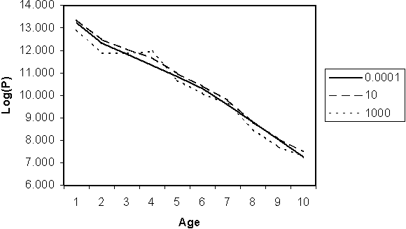
Notice that when the abundance index is not used, the difference between the observed and model catches can be reduced to zero. Including the abundance index produces a balance between the index and the catch link models in distributing the error between them. The balance is controlled by the lJ parameter (Figure 10.1), which is, essentially, the ratio between the variances of the catch and index series. As the lJ weight approaches zero, the standard VPA fits are reproduced as above. Conversely, as the parameter increases in size, the fit favours the abundance index, which the estimated population sizes will begin to resemble. Weighting heavily in favour of the index can lead to, for instance, increases in the population through time, essentially ignoring catches and the population model altogether. For this reason, the index is usually assumed to have lower weight compared to catches. If this is not the case, some other method will be needed to constrain the population size to realistic levels dictated by the population model.
This illustrates an important concept in stock assessment. The way the fishing activities impact the ecosystem in stock assessment is through catches. Other forms of impact, such as habitat degradation, need to be considered separately. Therefore, only catches appear in the population model. As long as they are correctly measured, fluctuations in population size brought about by fishing will be correctly determined. If they are not well measured, these fluctuations will add to the process errors. If fishing is having the largest single impact on the population, these introduced errors may be large, causing the results to be poor. Accurate catch data is therefore more important than effort or index data.
10.3.1 Separable VPA
10.3.2 Including Several Indices
Why combine cohorts into complicated-looking matrices rather than analyse each cohort separately? In the matrix form, the cohorts run diagonally through, each cohort remains entirely separate, and the models presented above could be fitted to each individually. Unless we build linkages across cohorts, there is no difference between fitting the VPA to separate cohorts and to the full cohort matrix. In matrix form, we can simply work back along each cohort, fitting each terminal F parameter separately. The reason for combining cohorts is to link the cohort models by sharing parameters between them. This will make parameter estimates more accurate.
As already mentioned, the plus-group can be modelled through multiple cohorts. This is of limited value, as the plus-group is usually chosen to be a trivial part of the catch. Of greater importance is to share any index parameters across cohorts. We are also able to construct new models, such as the separable VPA described below.
In separable VPA, we reduce the number of fishing mortality parameters by building a model of fishing mortality that applies across cohorts. This means the model no longer exactly fits and the exact solution to the Baranov catch equation no longer applies. Instead, we use the least-squares method to find the best fit between the observed (Table 10.7) and expected catches. In this formulation, the link model describes the relationship between the observed and expected catches, and the population model contains no data at all to drive it.
Table 10.7 Total catches recorded for all cohorts 1984-1994. Example catches used in the single cohort analyses above are highlighted by shaded cells.
|
Age |
1984 |
1985 |
1986 |
1987 |
1988 |
1989 |
1990 |
1991 |
1992 |
1993 |
1994 |
|
1 |
37937 |
25689 |
54983 |
96100 |
100014 |
155100 |
21200 |
56188 |
109213 |
36688 |
60240 |
|
2 |
27434 |
25608 |
17914 |
41556 |
68278 |
91377 |
114110 |
16660 |
42978 |
83706 |
36624 |
|
3 |
33684 |
31166 |
27537 |
16162 |
49154 |
81395 |
76090 |
81639 |
13066 |
29373 |
83690 |
|
4 |
20954 |
25082 |
22149 |
19460 |
14370 |
28193 |
48909 |
37360 |
53083 |
6860 |
26475 |
|
5 |
10266 |
11952 |
10270 |
21132 |
12784 |
9157 |
14879 |
29597 |
23121 |
32506 |
6124 |
|
6 |
6559 |
7698 |
8029 |
5790 |
7615 |
11391 |
5222 |
9278 |
14256 |
14064 |
24978 |
|
7 |
3161 |
3210 |
4936 |
4623 |
4786 |
6028 |
5618 |
2592 |
5001 |
8068 |
8544 |
|
8 |
1178 |
2062 |
2459 |
2568 |
2889 |
3182 |
2719 |
2641 |
1407 |
2706 |
4370 |
|
9 |
689 |
1116 |
1050 |
1349 |
929 |
1330 |
1410 |
1309 |
1253 |
643 |
1639 |
|
10 |
452 |
552 |
577 |
583 |
644 |
579 |
621 |
627 |
645 |
647 |
399 |
|
11+ |
453 |
545 |
628 |
616 |
643 |
789 |
586 |
608 |
569 |
576 |
726 |
 (128)
(128)
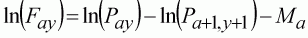
The Fay parameters now depend upon the separable VPA model:
 (129)
(129)
where Ey is the yearly exploitation rate. To avoid over-parameterisation, Ey can be chosen so that it is fishing mortality for the base age, and Sa represents relative departures from this level (Table 10.8), or similar methods. We can avoid the need for additional parameters by defining the terminal F parameters using the same model. So, for the current analysis:
 (130)
(130)
We could also use the estimated F11,y to define the plus-group population size in the same way, although this wastes the observed catch data for this group. Instead, we can define a model where this group accumulates survivors from the cohorts:
 (131)
(131)
Therefore, for any set of exploitation rates Ey and selectivity coefficients Sa, we can define the full matrix of population sizes and, more importantly catches through the Baranov catch equation. The task is to minimise the difference between these model log-catches and the observed log-catches by least-squares.
Comparing the estimated Fay to the true Fay generated by the simulation indicates much poorer estimates towards the end of the time series. This is always a problem with VPA techniques. The estimates are more accurate further back in time as there are more observations made on each of the cohorts. So, for example, the 1994 age 1 cohort has only one set of catches so the estimated F1,1994 is very unreliable. In contrast, the selectivity estimates, which makes use of data right across the matrix, are fairly good (Table 10.8).
Table 10.8 Fishing mortality estimated from the separable VPA model. The shaded cells contain the parameters used in the model and estimated by Solver. Comparison with the true parameters indiates that the selectivity is well estimated (r2=0.93) compared to the exploitation rate (r2=0.21).
|
Age |
1984 |
1985 |
1986 |
1987 |
1988 |
1989 |
1990 |
1991 |
1992 |
1993 |
1994 |
Sa |
Ma |
|
1 |
0.09 |
0.11 |
0.11 |
0.11 |
0.11 |
0.12 |
0.11 |
0.10 |
0.09 |
0.08 |
0.08 |
0.26 |
0.80 |
|
2 |
0.15 |
0.17 |
0.18 |
0.18 |
0.18 |
0.20 |
0.18 |
0.17 |
0.15 |
0.13 |
0.13 |
0.42 |
0.35 |
|
3 |
0.24 |
0.28 |
0.29 |
0.29 |
0.29 |
0.32 |
0.29 |
0.27 |
0.24 |
0.21 |
0.21 |
0.68 |
0.25 |
|
4 |
0.29 |
0.33 |
0.34 |
0.34 |
0.35 |
0.37 |
0.34 |
0.31 |
0.28 |
0.25 |
0.25 |
0.79 |
0.20 |
|
5 |
0.32 |
0.37 |
0.38 |
0.38 |
0.38 |
0.41 |
0.38 |
0.35 |
0.31 |
0.28 |
0.28 |
0.88 |
0.20 |
|
6 |
0.35 |
0.41 |
0.42 |
0.42 |
0.43 |
0.46 |
0.42 |
0.39 |
0.34 |
0.31 |
0.31 |
0.98 |
0.20 |
|
7 |
0.36 |
0.41 |
0.43 |
0.43 |
0.43 |
0.47 |
0.43 |
0.40 |
0.35 |
0.31 |
0.31 |
1.00 |
0.20 |
|
8 |
0.36 |
0.41 |
0.42 |
0.43 |
0.43 |
0.46 |
0.42 |
0.39 |
0.35 |
0.31 |
0.31 |
0.99 |
0.20 |
|
9 |
0.37 |
0.43 |
0.44 |
0.44 |
0.45 |
0.48 |
0.44 |
0.41 |
0.36 |
0.32 |
0.32 |
1.03 |
0.20 |
|
10 |
0.36 |
0.41 |
0.43 |
0.43 |
0.44 |
0.47 |
0.43 |
0.40 |
0.35 |
0.31 |
0.31 |
|
0.20 |
|
11+ |
0.31 |
0.36 |
0.37 |
0.37 |
0.38 |
0.40 |
0.37 |
0.34 |
0.30 |
0.27 |
0.27 |
0.86 |
0.20 |
For variety, we develop a slightly different model, based upon the classical VPA population model. The same parameter set up as in Table 10.8 is used for fishing mortality. For the population model, however, we use the observed catches solving the standard VPA equation:
 (132)
(132)
For the terminal populations, we use the terminal F estimate (Equation 130) and back-calculate cohorts by solving Equation 132. However, as the plus-group accepts cohorts from the terminal population (age 10), we must use the forward VPA solution to estimate this population, adding together both the survivors from the previous year’s plus group and the survivors from the new cohort (last year’s age 10). For each age group in each year, we can now minimise the squared difference between the population model estimate of the log-Fay with the separable estimate of the log-Fay.
With effort data replacing the exploitation rate, only selectivity (Sa) needs to be estimated. This results in the population and fishing mortality being estimated reasonably well with only 10 parameters (Table 10.9). Although this separable VPA model was used in the simulation to generate the data, both fishing mortality and catch were estimated as log-normal variates, so the error remains high. As in the previous models, errors were worse for the more recent years, the ones that are usually of most interest. This problem can really only be addressed using other sources of data.
Table 10.9 Fishing mortality estimated from the separable VPA model with effort data. The shaded cells contain the parameters used in the model and estimated by Solver. The exploitation rate is now correct as it uses the simulation effort data. Comparison with the true selectivity parameters indicates the selectivity is well estimated (r2=0.88). The overall F estimates are much better than when the exploitation rate was unknown, but the most inaccurate estimates remain in 1994 year.
|
|
1984 |
1985 |
1986 |
1987 |
1988 |
1989 |
1990 |
1991 |
1992 |
1993 |
1994 |
Sa |
|
Effort |
2100 |
2200 |
2200 |
2300 |
2500 |
3000 |
2900 |
2900 |
2900 |
2900 |
4000 |
|
|
Age 1 |
0.08 |
0.09 |
0.09 |
0.09 |
0.10 |
0.12 |
0.12 |
0.12 |
0.12 |
0.12 |
0.16 |
4.00 10-5 |
|
2 |
0.14 |
0.14 |
0.14 |
0.15 |
0.16 |
0.19 |
0.19 |
0.19 |
0.19 |
0.19 |
0.26 |
6.48 10-5 |
|
3 |
0.22 |
0.23 |
0.23 |
0.24 |
0.26 |
0.32 |
0.31 |
0.31 |
0.31 |
0.31 |
0.42 |
1.05 10-4 |
|
4 |
0.26 |
0.27 |
0.27 |
0.28 |
0.31 |
0.37 |
0.35 |
0.35 |
0.35 |
0.35 |
0.49 |
1.22 10-4 |
|
5 |
0.28 |
0.29 |
0.29 |
0.31 |
0.33 |
0.40 |
0.39 |
0.39 |
0.39 |
0.39 |
0.53 |
1.33 10-4 |
|
6 |
0.30 |
0.32 |
0.32 |
0.33 |
0.36 |
0.43 |
0.42 |
0.42 |
0.42 |
0.42 |
0.58 |
1.45 10-4 |
|
7 |
0.33 |
0.35 |
0.35 |
0.36 |
0.39 |
0.47 |
0.46 |
0.46 |
0.46 |
0.46 |
0.63 |
1.57 10-4 |
|
8 |
0.34 |
0.36 |
0.36 |
0.38 |
0.41 |
0.49 |
0.48 |
0.48 |
0.48 |
0.48 |
0.66 |
1.64 10-4 |
|
9 |
0.33 |
0.34 |
0.34 |
0.36 |
0.39 |
0.47 |
0.45 |
0.45 |
0.45 |
0.45 |
0.62 |
1.55 10-4 |
|
10 |
0.33 |
0.34 |
0.34 |
0.36 |
0.39 |
0.47 |
0.45 |
0.45 |
0.45 |
0.45 |
0.62 |
1.56 10-4 |
|
11+ |
0.25 |
0.26 |
0.26 |
0.28 |
0.30 |
0.36 |
0.35 |
0.35 |
0.35 |
0.35 |
0.48 |
1.20 10-4 |
We now consider the case where we have three indices of abundance. In addition to a scientific survey, as used for the single cohort, we assume we have a biomass index and the effort data used in the previous example. Rather than construct a new model, we shall use the separable VPA analysis with effort data described above (Section 10.3.1). The approach is much the same for several abundance indices as for one, however each index may have a different model linking it to the population.
For the scientific survey, we assume that sampling was organised such that we can have confidence that the relationship between the index and cohort size in each year is linear and errors are log-normal:
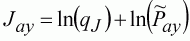 (133)
(133)
The timing for the index will be the third quarter of the year. The least-squares estimate of the coefficient ln(qJ) can be calculated using the normal linear least-squares techniques. In this case, the solution is very simple, it is the average difference between the log-population size and the index:
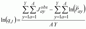 (134)
(134)
We will imagine here that for the biomass index only catch weight per unit effort data were recorded, so it is related to the total biomass of the population in the year. Hence,
 (135)
(135)
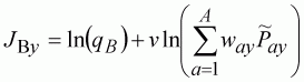
where way is the average weight at age in each year. Weight data would probably be available from the scientific survey and catch samples. The biomass index could be obtained from another scientific survey using fishing gear or from an acoustic survey. Note that in this case we do not assume a linear relationship between the index and population size. This might be because, for example, the data was a by-product of a survey for another species, not designed to sample this species, rendering the linear relationship suspect. Also note that it may be possible to obtain, through acoustic surveys for example, an absolute estimate of the biomass which would not require an estimate of ln(qB) or v. This is highly desirable as it reduces the parameters required and more importantly parameter aliasing.
Once we have calculated the population sizes at the time of the survey, and we know the average size of each age group, for any set of population parameters we can calculate the biomass in each year. This is the x2 variable in the regression. The x1 variable is a dummy variable for the constant term. Given the observed index, we can find the least squares solution directly by inverting the Hessian matrix. As the matrix is small, we can write out the full equations for the least-squares estimates:
 (136)
(136)
Finally, we consider using the effort data. As will have been gathered, effort can be included in the assessment in a variety of ways. Perhaps most commonly, we can produce CPUE as abundance indices, and use models similar to the scientific survey or biomass link models (Equations 133 or 135). However, it is important to appreciate the variety of approaches available that may be used to adapt techniques to local fisheries and data sets. To illustrate alternatives, we use the separable VPA model to build a link between the population and the observed effort. We reverse the log form of the separable VPA model (Equation 129) to generate the expected exploitation rate from the model:
 (137)
(137)
This can be compared with the observed effort in each year. The Fay can be calculated for each age and year by:
 (138)
(138)
with the exception of the terminal years. For these, where Pa+1,y+1 is unavailable, we need to solve the Baranov catch equation for F calculating forward (see Macro 10.2). Once we have the Fay matrix, the least-squares solution for Sa parameters can be calculated as the mean difference between the log-effort and log-fishing mortality:
 (139)
(139)
The aim now is to minimise the least-squares equation:
 (140)
(140)
As well as the link model parameters, qJ, qB, v and Sa, we need to estimate the full set of VPA terminal population parameters PAy and PaY. In addition, we need the relative weights for the series: lJ, lB. Note that even if we are particularly interested in forecasting based on projected effort data, we gain no advantage from weighting the model in favour of the effort index. Incorrect weighting will simply lead to a poorer model, which will produce poorer forecasts. For simplicity, here we assume lJ = lB = 1.0. In a real stock assessment, these relative weights might be the subject of much discussion.
We now fit the model using a two level iterative process. At the outer level, the population model is fitted in the usual way, by using a non-linear numerical optimiser altering the terminal population sizes to minimise the least squares. At the inner level, the link models can be estimated using linear least-squares techniques in one iteration.
Macro 10.2 This Visual Basic macro solves the VPA equation for logeFa using the Newton-Raphson method and parameters Ma, catch and Pa. The method is inherently less stable than others presented here, so the function includes additional checks. In particular, if the convergence is very slow, the method tries to leap towards the solution by bisection. This avoids problems such as oscillating around the solution.
|
Function SolFVPAF(M, Ca, Na_1 As Double) As Double |
||||
|
Dim fx, dfx, C, DeltaD, OldDeltaD, Z, F, G, D As
Double |
||||
|
|
‘Estimate initial F from Pope’s cohort
equation |
|||
|
G = Na_1 - Ca * Exp(M / 2) |
|
|||
|
If (Na_1 <= 0) Or (G < 0) Then |
|
|||
|
|
SolFVPAF = Log(10) ‘ |
Return very high F - we’re catching fish that aren’t
there! |
||
|
Else |
|
|||
|
|
D = Log(Log(Na_1) - Log(G)) |
|
||
|
|
Do |
|
||
|
|
|
F = Exp(D) |
‘Current F |
|
|
|
|
Z = F + M |
‘Calculate total mortality |
|
|
|
|
G = (1 - Exp(-Z)) |
‘Temp calculation variable |
|
|
|
|
C = F * Na_1 * G / Z |
‘Catch for current F |
|
|
|
|
fx = Ca - C |
‘Calculate the function |
|
|
|
|
dfx = C * (M * G / Z + F * Exp(-Z) / G) |
‘And its -derivative |
|
|
|
|
DeltaD = fx / dfx |
‘Calculate the new correction factor |
|
|
|
|
D = D + DeltaD |
‘Add it to LogF |
|
|
|
|
If DeltaD < 0.00005 Then Exit Do |
‘Test for accuracy |
|
|
|
|
If (OldDeltaD - Abs(DeltaD)) < 0.0000001 Then |
‘Test for convergence |
|
|
|
|
|
D = D - DeltaD / 2 |
‘No covergence, so guess a new value by
bisection |
|
|
End If |
|
||
|
|
OldDeltaD = Abs(DeltaD) |
|
||
|
|
Loop |
|
||
|
|
SolFVPAF = D |
‘Return solution |
||
|
End If |
|
|||
|
End Function |
|
|||
|
Age |
1984 |
1985 |
1986 |
1987 |
1988 |
1989 |
1990 |
1991 |
1992 |
1993 |
1994 |
|
1 |
561501 |
345337 |
737407 |
1233835 |
1186411 |
1551036 |
219413 |
579325 |
1152034 |
386663 |
518020 |
|
2 |
252595 |
187756 |
120946 |
237081 |
362551 |
348188 |
411557 |
72348 |
188272 |
306028 |
107001 |
|
3 |
138760 |
146470 |
107819 |
67705 |
130088 |
191258 |
147423 |
161412 |
28023 |
58141 |
93519 |
|
4 |
77549 |
81545 |
91182 |
66221 |
41515 |
68455 |
79064 |
66097 |
66273 |
11797 |
16164 |
|
5 |
42983 |
50764 |
50727 |
61173 |
43668 |
20940 |
27733 |
35137 |
26938 |
24016 |
2832 |
|
6 |
24017 |
30379 |
34569 |
34816 |
37783 |
24244 |
8642 |
12442 |
13834 |
10643 |
5973 |
|
7 |
9807 |
17194 |
21081 |
23784 |
24539 |
21843 |
10872 |
3653 |
4686 |
5264 |
3044 |
|
8 |
3780 |
6993 |
12450 |
14584 |
16150 |
12313 |
7433 |
4498 |
1550 |
1977 |
1303 |
|
9 |
1632 |
2776 |
4915 |
8632 |
9955 |
9002 |
5817 |
2775 |
1900 |
657 |
561 |
|
10 |
1022 |
1177 |
1843 |
3490 |
6137 |
5650 |
4148 |
1639 |
1071 |
602 |
231 |
|
11 |
381 |
976 |
1435 |
2027 |
3272 |
4789 |
3562 |
2531 |
1523 |
740 |
344 |
The parameters fed to the optimiser form part of the population model (Table 10.10). There is a danger that the optimiser will attempt to try parameters that are impossible (even if these values are excluded by the constraints within the optimiser!). Once a function returns an error the optimiser will stop, so we need to catch the errors before they occur. The main problem here is that the optimiser will try terminal population sizes, which do not cover the catches in that year. While the VPA functions (e.g. Macro 10.2) may capture these invalid values, we really need to ensure they never enter the model. This can be done by using “IF()” functions as part of the spreadsheet cell calculation. So, for example, in Excel the terminal population size of Age 1 1994 in Table 10.10 could consist of:
|
=IF(P23<N5*EXP($K5/2),N5*EXP($K5/2),P23) |
|
=IF(R24<(E14+F15*EXP($K14))*EXP($K14/2),(E14+F15*EXP($K14))*EXP($K14/2),R24) |
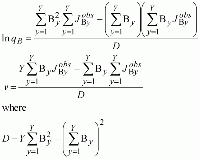
Table 10.11 Biomass and biomass indices for fitting the population model. The link model here is linear, so the parameters are calculated by a regression between the x (population model biomass) and y (observed index) variables. The calculations can be carried out using the Equations 67 or by inverting the Hessian matrix (see below), the two methods being equivalent. Notice that the parameter covariance matrix indicates that the correlation between the parameters is very high, so the estimates are inaccurate (The true value for v is 0.4). The results indicate that the v parameter is redundant and could be excluded. However, as the parameters are not going to be used, there purpose being purely to account for variation due to the measurement, it will make little difference in this case.
|
|
1984 |
1985 |
1986 |
1987 |
1988 |
1989 |
1990 |
1991 |
1992 |
1993 |
1994 |
|
|
Biomass |
13.319 |
13.312 |
13.375 |
13.506 |
13.593 |
13.767 |
13.631 |
13.627 |
13.674 |
13.543 |
13.434 |
|
|
|
Index |
|
|
|
|
|
|
|
|
|
|
|
|
|
Model |
21.794 |
21.576 |
23.565 |
27.754 |
30.527 |
36.072 |
31.745 |
31.607 |
33.123 |
28.920 |
25.465 |
|
Obs |
20.207 |
22.361 |
24.055 |
27.812 |
30.705 |
36.337 |
31.857 |
31.643 |
32.447 |
28.506 |
26.219 |
|
|
Residual |
2.520 |
0.616 |
0.240 |
0.003 |
0.032 |
0.070 |
0.013 |
0.001 |
0.458 |
0.172 |
0.569 |
|
|
|
|
|
|
|
|
|
|
|
Sums of Squares |
4.693 |
|
|
|
Hessian |
Covariance |
|
|
|
|
||||
|
|
11 148.78 |
|
809.459 |
-59.840 |
yx1 |
312.15 |
|
ln(qB) |
-403.11 |
|
|
148.78 2012.56 |
|
-59.840 |
4.424 |
yx2 |
4229.19 |
|
v |
31.90 |
|
Determinant 2.486 |
|
Correlation -0.9999 |
|
|
|
|
|
||
Using generalised linear models, we can build quite complex link model structures into stock assessment, handling a larger number of parameters than would otherwise be possible. Traditionally, analyses of variables, which might be used in stock assessment are carried out as separate exercises, and only the results are carried forward to the stock assessment. For example, only the year terms of a linear model describing the CPUE of a number of fleets might be used as indices of abundance, the remaining information in the data series being discarded. Although this sequential approach makes analysis easier, it will not be clear how the models interfere with each other and whether information is being discarded which is useful. Explanatory variables may remove variability in the data with which they are correlated, which could be indicators of population changes. It is therefore worth considering carrying out an analysis of the complete model wherever possible. This has largely been avoided simply due to the technical difficulties of fitting models with large numbers of parameters. By carefully structuring models, these problems can often be avoided.
Incorporating linear models suggests an approach to further analysis and simplification. In the biomass link model used previously (Table 10.11), it was found that the qB and v parameters were too heavily correlated to estimate together. The number of parameters in the linear model therefore could be reduced without significant loss to the model’s efficacy. In general, linear regression, analysis of variance and analysis of covariance use analysis of variance tables to make these decisions. We can use similar tables to summarise information about covariates and their power to explain underlying population changes.
In the following example we try to model the fleet structure, testing for differences among vessels using a linear model. It is quite possible to develop much more sophisticated models than that discussed here. In particular, we could use log-linear models to account for changes in catchability alongside population size (McCullagh and Nelder 1983).
Instead of having one fleet, we consider now the case where the fleet is known to be divided in two, a predominantly inshore fleet of small boats, and an offshore fleet of industrial vessels. We wish to know what different effects these fleets have on the stocks. The individual catches and effort of the fleets are available. We can extend the model of fishing effort above to allow for differences between fleets and see if these differences better explain changes in the fishing mortality.
There are essentially five models linking fleets to fishing mortality, based on whether age selectivity is present and whether the fleets have different catchabilities. In general form, the optional link models can be set out as:
 (141)
(141)
where subscript 2 refers to the parameter measuring differences between the two fleets, and subscript a refers to parameters measuring catchability by age. Hence, the first two models do not differentiate catchabilities between ages, whereas the first and third models do not differentiate between fleets. The fourth model allows the fleets to have different catchabilities, but assumes that the selectivity is proportionally the same. The fifth model allows different catchabilities for both fleets as well as ages. The terms 1, A and G refer to the constant, age and fleet effects representing the models in standard generalised linear model (GLM) form. In GLMs, S1a and S2b could be formulated as linear predictors for the catchabilities in a multiplicative model. We would need to implement an iterative weighted least-squares method to allow alternative likelihoods besides the log-normal. In this case however, we can find the least-squares estimates by calculation as the models are assumed log-normal.
By fitting the whole model with each different link model and recording the sum of squares, we can build up an ANOVA table (Table 10.12). The ANOVA table tests how much worse each model does compared to the full model where parameters are fitted to allow for age and fleet differences. It is useful, although not always practical, if the full model, including the population model, is fitted for each link model to generate the sum of squares, as parameters in the link model may be just as well explained as changes in the population size. If it is found that the population model parameters change significantly as the link model is changed, but the sum of squares does not, then there is evidence of conflicting hypotheses, viz. either there are changes in the observations or changes in the population. Without other evidence, the precautionary approach requires assuming the worst hypothesis, even if it requires more parameters. Otherwise, the model with the smallest number of parameters should be chosen as the best model.
Table 10.12 ANOVA for the fleet link model. The sums of squares are shown for models with increasing numbers of parameters. All models are compared to the fully parameterised model as we would wish to test which terms we can safely remove as they do not explain significant amounts of the variation. The full model is used to estimate the error sums of squares. We can calculate the F statistic as the ratio between the mean square of each model and the error. Those models which show very small F-statistics are equivalent to the full model, and of this group the “worst case” model with the smallest number of parameters should be chosen. In this case, the S1a model is almost equivalent to the full model, indicating that there are no significant differences between fleets. However, as soon as we assume that selectivity does not change between ages (S1, S1+S2) the model gets significantly worse. Note the approximate F-statistic here may not be distributed as the F-statistic in statistical tables unless the errors are truly normally distributed. However, it can still be used for guidance.
|
Model |
SS |
Change |
df |
MS |
F Statistic |
|
S1 |
30.171 |
7.729 |
21 |
0.368 |
5.379 |
|
S1+S2 |
30.164 |
7.722 |
20 |
0.386 |
5.643 |
|
S1a |
22.722 |
0.279 |
11 |
0.025 |
0.371 |
|
S1a+S2 |
22.721 |
0.279 |
10 |
0.028 |
0.407 |
|
S1a+S2a (Error) |
22.442 |
|
328 |
0.068 |
|
Using ANOVA techniques with these types of non-linear models is potentially dangerous if the statistics are taken too literally. Even if errors are normally distributed, we might expect structural errors to be more severe where linearity cannot be assumed. Nevertheless, calculating statistics based on measures of goodness-of-fit is still very useful in summarising the value of parameters and whole sub-models in explaining variation in the observations even if strict hypothesis testing cannot be reliably conducted.
10.5.1 Fitting the Model
10.5.2 Indicators and Reference Points
It may often be the case that several sets of distinct data will have implications on the same parameters. For example, total catch age composition may be available from commercial sources, as well as more detailed sampled data, perhaps from an observer programme. It is often of interest to link the parameters to both sources of data simultaneously to obtain the best estimates possible.
The problem with separate models linking to parameters of interest is that the data may be in quite different forms. If this is the case, we firstly have to identify some common model, which can be used to develop the links. Likelihood is a useful concept in sorting these issues out. The common ground in likelihood is probability, so all data are compatible across likelihood models, and log-likelihoods can be added. This forms the basis for summing weighted sums-of-squares.
When combining sums-of-squares, it helps to be aware of the underlying likelihood models to ensure we make the correct sum. Broadly, this can be done by converting different data series so that their x-variables are compatible, and so all data can be written in a single matrix form. Although you may not actually write out the matrix, you ideally should be clear on how it should be done, as these calculations will form the basis of the data conversion to make it compatible. Often the best way to approach this problem is to consider the original raw data from which the data you have are derived. The raw data themselves may not be available, nevertheless you should be aware of the common fundamental data units (catch per haul, box of commercial groups, vessel landings etc.) from which several data have been derived.
In the following example, a more realistic data set and analysis is developed. The population model and survey data remain the same as used in the above analyses, however we add data taken from a detailed observer survey of commercial vessels which was designed to estimate the impact of new gear technology.
The observer survey was carried out in the same month of 1993 and 1994 and took detailed records of the catch-at-age as well as the gear on board the vessel. The survey was designed to cover vessels with and without two improvements in gear (GPS and monofilament nets) to estimate potential changes in catchability. Under normal circumstances, we would use linear models to estimate the relative change in CPUE due to the different gear use. This would estimate the relative fishing powers, which would be used as fixed adjustments in the stock assessment. However, by doing the analyses sequentially, we would automatically be assuming that all the observed correlation between different gear use and catch rates can be assumed to be due to the gear, not changes in the underlying population size. If this is incorrect, the analysis will be removing useful information from the data without our being aware of the implications to the stock assessment. For this reason, it is always better to try doing the analysis in a single combined model wherever possible.
In the previous analysis, we included the population model when testing whether particular parameters were useful in explaining variation in the data, so we could reduce the model to the most parsimonious possible. This is the preferred method, but it can be very time consuming when not using specialist software. Often this approach is unnecessary for choosing the parameters that will be needed. In this case, a separate linear model analysis on the catch rates should be adequate to identify which parameters are correlated as long as we remove the effective population size for each age group in each year. This can be done by fitting these effects as a minimum model in generalised linear model analysis. Specialist software can then be used to test alternative models, in particular whether factors interact.
Interaction effects are important, and occur where two independent variables together produce a different effect than simply the sum of their independent effects. For example, GPS may have a disproportionately larger effect on vessels also possessing the improved gear design than on those that do not. Significant interaction effects will lead to a large increase in the number of parameters required by the linear model, as interactions are multiplicative. For example, the number of parameters required to estimate the effect of GPS which does not interact with selectivity would be 12, whereas a significant effect would require 22 parameters, enough to fit two separate selectivities with and without GPS.
While these analyses can be carried out in spreadsheets, interaction effects between discrete factors (such as fleet and gear types) require large numbers of dummy variables to be generated for the different models. This is very time consuming in spreadsheets, whereas specialist statistical software handles these effects automatically. As long as potential effects from population changes can be accounted for, this approach may be preferred in choosing the final model which should be fitted, or at least reducing the number of models to be tested.
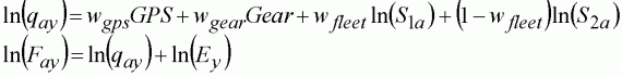
In this example, we assume that no significant interaction effects were found between gears and fleets, and gears and selectivity, but that each fleet was found to take a significantly different age composition. The model to be fitted has terms for GPS, monofilament and selectivity by fleet, i.e. 24 parameters. So for a particular survey observation, i, the expected catch-at-age can be described by:
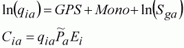 (142)
(142)
where the GPS and Mono terms are present when those gear were used on the observed vessel, and g indicates the fleet to which the vessel belongs. Because we use logarithms of the data, we assume that the errors are normally distributed and that the model is multiplicative. However, in a few instances catches were zero. To avoid problems with this, we added a constant to catch data.
We also have a time series of effort data, and the proportion of GPS and monofilament in the fleets since 1984. We wish to estimate simultaneously the GPS, Gear and fleet selectivity parameters for both the observer vessel survey and total effort.
In simulations, it is easy to assume some level of convenience in what data the scientist possesses. For instance, in the previous example we happen to have catches separated by fleet. In practice, data, or the lack of it, is usually the main problem in the analysis. In this scenario, it is assumed we neither have catches separated by fleet nor gear type, only age. However, if we at least know the proportional gear use, we can still calculate the expected fishing mortality in each year as the weighted average of the fleet combined.
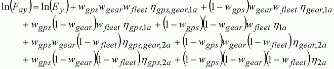
 (143)
(143)
where the weights, w, are the proportion of the fleets in each category. Notice that although the linear model is the same as Equation 142, the catchability is linked to the fishing mortality rather than population size. Equation 142 can be fitted as long as we have the weights, total effort and fishing mortality.
The two catchabilities in Equations 142 and 143 will be equivalent as long as the survey observation lasts a short time. Although any change in population size during the survey observation will introduce a structural error between the two models, this difference is unlikely to be significant if the time period is small. Both models are only approximations to reality. For example, the fishing mortality model assumes a constant exploitation rate during the period it applies and an instantaneous reaction from catch rates to removals. The difference model, relating average stock size to catch rates over a fixed period assumes a delay between removals and catch rate change, and the change is a step function. Neither is strictly correct.
The fitting procedure for Equations 142 and 143 is more difficult than those previously discussed. One option is to use a non-linear standard fitting routine, finding the least squares solution to fitting the observed and expected mean log CPUE for the survey data (by manipulating Equation 142) and mean log total yearly effort (defined by manipulating Equation 143). Although this is fine for the survey data, it produces an incorrect result for the effort model. This is because the least squares solution for effort model is incorrect as we have not considered all combinations of the vessel characteristics from which observed mean fishing mortality has been derived. We first assume gears are distributed among categories proportionally. So if 20% of all vessels possess GPS, also 20% of the vessels in fleet group 2 using monofilament have GPS. Under these circumstances, the mean log fishing mortality of age a fish is:
 (144)
(144)
where hgps,gear,1a indicates the linear predictor with terms GPS, Gear and fleet-age (S1a) as in Equation 143. Adding over the terms, the mean is exactly the same as that in Equation 143. But the contribution of the individual fleet categories to the sum-of-squares is different:
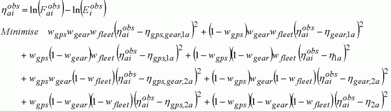 (145)
(145)
where h is the model linear predictor,
e.g. 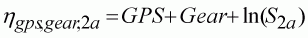
Hence Equations 143 and 144 only give the least-squares estimate of the log fishing mortality per unit effort for hmod as if it were a single parameter, but not the individual parameters that make up the linear predictor. Correct fitting for the individual parameters requires consideration of all combinations of attributes parameterised in the model. The weights refer to the inverse variance of the estimated catch rate within each category, rather than a contribution to a mean value. We need to calculate correctly the sum-of-squares so that we can combine with information from other sources, and for this, the full weighted combinations are necessary.
This illustrates an important point. Often statistics are taught covering simple procedures where underlying assumptions are implicit. In real-world problems of fisheries, some assumptions may well turn out to be incorrect. It is therefore always worthwhile returning to the basic procedures and checking which simplifying assumptions may be used. Although not directly observed, the fundamental data are the individual vessel catches per unit effort (y-variable) and the gear they possess (x-variables). This is essentially the data we have from the scientific vessel survey. From this simple point, we need to develop a model of how the observed variables, the annual fishing mortality per age per unit effort, would arise. To do this, we could gather all individual observations into groups with the x-variable combinations (i.e. gear), and calculate the average y-variable and the weighting factor for each group. This is essentially, Equation 145. What you would not do is add up the catch rates of all the vessels with each gear type into groups, as vessels with more than one gear type would appear in more than one group. This is what we would be doing if we used Equation 143 as the basis for an estimator.
The GPS, Gear (monofilament) and fleet selectivities are discrete factors and must be represented in fitting the model as dummy variables. Dummy variables take on a value of one when its parameter applies and zero when it does not apply (
Table 10.13). The x-variables, can, as in this case, consist solely of binary values. Analysis of variance and covariance are based on this type of model. Once we have generated a full data matrix of all fleet-gear combinations in each year, joined to the same format matrix for the survey observations, we can multiply the data matrix (n observations on m x-variables) by a parameter vector (m estimates) to produce a vector of expected values of qia (length
n). We can calculate the sum-of-squares comparing the expected qia with the observed calculated from the log CPUE and population size for the survey, and the expected qia with the observed calculated from the log fishing mortality and total effort. We add this sum-of-squares to the sums-of-squares from the scientific resource survey and can pass this total sum to an optimiser to minimise with respect to the terminal population sizes and the linear model. If you do this, despite having 45 parameters and a data matrix length of over 1000 observations, the optimiser should be able to find the minimum reasonably quickly, 5-10 minutes on a fast desktop computer. Optimisers in general will do reasonably well, as they often assume linearity to find trial solutions (as in the Hessian matrix), so the 24 parameters belonging to the linear model do not prove too great an obstacle. Even if you try to improve on this approach, it may be worthwhile to estimate values this way initially. As you set up more complicated but more efficient approaches, you can then ensure the method is correct as the resulting estimates should be very close if not exactly the same.
Table 10.13 Example dummy for two observations. One of a vessel of fleet type 1 with GPS, but not the improved gear design and another of a vessel of fleet type 2 with GPS and improved gear. The age class of the catch is a discrete factor variable with 11 levels. Unlike the GPS and Gear terms, these are mutually exclusive, so a vessel can either be of type 1 or 2, but not both and the catch can be of only one age. The data set possesses catch and effort covariates. Catch will vary with age categories, but effort will remain constant across a single survey observation. The number of columns, GPS to Age (S2a) 11 is the same as the number of parameters required by the model.
|
Year |
GPS |
Gear |
Age (S1a) |
Age (S2a) |
||||||||||||||||||||
|
1 |
2 |
3 |
4 |
5 |
6 |
7 |
8 |
9 |
10 |
11 |
1 |
2 |
3 |
4 |
5 |
6 |
7 |
8 |
9 |
10 |
11 |
|||
|
1993 |
1 |
0 |
1 |
0 |
0 |
0 |
0 |
0 |
0 |
0 |
0 |
0 |
0 |
0 |
0 |
0 |
0 |
0 |
0 |
0 |
0 |
0 |
0 |
0 |
|
1993 |
1 |
0 |
0 |
1 |
0 |
0 |
0 |
0 |
0 |
0 |
0 |
0 |
0 |
0 |
0 |
0 |
0 |
0 |
0 |
0 |
0 |
0 |
0 |
0 |
|
1993 |
1 |
0 |
0 |
0 |
1 |
0 |
0 |
0 |
0 |
0 |
0 |
0 |
0 |
0 |
0 |
0 |
0 |
0 |
0 |
0 |
0 |
0 |
0 |
0 |
|
1993 |
1 |
0 |
0 |
0 |
0 |
1 |
0 |
0 |
0 |
0 |
0 |
0 |
0 |
0 |
0 |
0 |
0 |
0 |
0 |
0 |
0 |
0 |
0 |
0 |
|
1993 |
1 |
0 |
0 |
0 |
0 |
0 |
1 |
0 |
0 |
0 |
0 |
0 |
0 |
0 |
0 |
0 |
0 |
0 |
0 |
0 |
0 |
0 |
0 |
0 |
|
1993 |
1 |
1 |
0 |
0 |
0 |
0 |
0 |
0 |
0 |
0 |
0 |
0 |
0 |
1 |
0 |
0 |
0 |
0 |
0 |
0 |
0 |
0 |
0 |
0 |
|
1993 |
1 |
1 |
0 |
0 |
0 |
0 |
0 |
0 |
0 |
0 |
0 |
0 |
0 |
0 |
1 |
0 |
0 |
0 |
0 |
0 |
0 |
0 |
0 |
0 |
|
1993 |
1 |
1 |
0 |
0 |
0 |
0 |
0 |
0 |
0 |
0 |
0 |
0 |
0 |
0 |
0 |
1 |
0 |
0 |
0 |
0 |
0 |
0 |
0 |
0 |
|
1993 |
1 |
1 |
0 |
0 |
0 |
0 |
0 |
0 |
0 |
0 |
0 |
0 |
0 |
0 |
0 |
0 |
1 |
0 |
0 |
0 |
0 |
0 |
0 |
0 |
|
1993 |
1 |
1 |
0 |
0 |
0 |
0 |
0 |
0 |
0 |
0 |
0 |
0 |
0 |
0 |
0 |
0 |
0 |
1 |
0 |
0 |
0 |
0 |
0 |
0 |
|
1993 |
1 |
1 |
0 |
0 |
0 |
0 |
0 |
0 |
0 |
0 |
0 |
0 |
0 |
0 |
0 |
0 |
0 |
0 |
1 |
0 |
0 |
0 |
0 |
0 |
- Building the matrix: The number of factors and matrix structure may have to be generated. Given the size of the matrix, this may require a great deal of typing and copying values and may make it easy to introduce mistakes. In this case, we can generate the sums-of-squares more directly than using dummy variables because the weights are multiplicative. If there were different weights for each gear-catch combination category, we may still have to generate the full matrix.10.5.1.1 Using Weights- Computer memory inadequate: The matrix length for the total effort model would account for 2 fleets, 2 gears, 2 GPS, 11 age and 11 year categories, producing a grand total of 968 rows in the matrix (to estimate only 11 effort values!). For more interaction terms, the number of rows would be much larger than this and easily overflow memory on smaller computers. However, it is relatively easy to produce the Hessian (information) matrix, which has the same length as the number of parameters and holds all the information necessary for finding the least squares solution in the linear model.
- Speed of calculation: This is probably the most important issue. While 10 minutes computing time for one fit seems short, it very soon adds up. A proper stock assessment will always need to assess how robust the results are to changes in assumptions, and therefore a number of fits are required to test sensitivity. Even after you are satisfied with the model, the chances are that you will wish to generate bootstrap estimates for confidence intervals and other statistics. If you require 1000 bootstrap estimates, each taking 10 minutes, it will take about 7 days to get an adequate number. Since Murphy’s Law invariably means you find you have forgotten to divide some critical value by 2 after completing 500 bootstraps, reducing this time to a minimum is important. This can be done both by reducing the size of the matrix and solving the linear model directly, by-passing the non-linear optimising routine.
Using weights is often the simplest way to reduce the size of data sets without losing pertinent information. All data records which possess the same x-variable values can be combined in this way. The use of weights is underpinned by the assumption of normal errors, and is strictly the inverse variance of the y-variable. However, the method is more generally valid as long as the weights represent the relative changes in variance of the y-variable.
In any case where raw data records are combined, weights should be considered to account for changes in variance. For the observer data, the original form of data was daily records. These were combined into total catch and effort by vessel. If the log-catch on each day is normally distributed, the variances will be additive, so the variance of the total values will be proportional to the number of observations (i.e. the effort) that are combined to make them. If the model and relative variances are correct, the relevant information in the data for estimating least squares can be maintained in a smaller data matrix with totals and weights. However, it is worth confirming the weighting is correct, by examining model residuals, ensuring they show variation consistent with their weights.
10.5.1.2 Solving Linear Sub-Models
Probably the most robust method for solving linear least-squares problems is Singular Value Decomposition (SVD). SVD will decompose a data matrix into a form that allows a solution to be found to the simultaneous differential equations very rapidly. There are several advantages to this approach.
· The least-squares estimates are more accurate than those obtained from a non-linear optimiser and take less time to solve.10.5.1.3 Using the Linear Information Matrix· If only the y-variable changes, the least-squares parameter estimates can be found without having to decompose the matrix again. This is very useful in this context, where only the y-variable is affected by changes in the population size. If you are able to construct your models in this form, where the x-variables and weights do not change, SVD offers considerable increases in speed as well as reliability.
The Hessian matrix in linear regression is often known as the information matrix. It summarises the data with respect to the x-variables, and with the xy-vector represents the normal equations, which solve the least-squares problem. SVD also works on the information matrix as well as the data matrix. The information matrix is a square matrix with length of sides equal to the number of parameters. Calculation of the information matrix where it is relatively fast, or only has to be carried out once, may reduce both memory use and calculation time in finding least-squares solutions. However, if the solution is nearly singular (i.e. parameters aliased or too heavily correlated), using the information matrix may increase instability of the results.
Each cell in the linear information matrix is the sum of the products of pair of x-variables as identified by the row, j, and column, k, and each row in the xy-vector is the sum of the product of the jth x-variable times the y-variable.
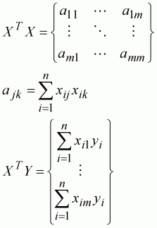 (146)
(146)
The x2 variables are making up the diagonal of the information matrix, and the matrix will be symmetric (akj = ajk). To take as an example the observer survey model (Table 10.14), Equation 146 consists of multiples of dummy variables, which indicate whether a vessel possesses a particular gear, or the age group of the catch. So matrix term a11 is the number of all observations possessing GPS and a12 is the number of all observations possessing both GPS and the new improved gear. An observation is the catch of a particular age group by a vessel of either fleet 1 or fleet 2. Age groups and fleets are mutually exclusive, so most of the cells, such as a34 to a3,24, are zero. If we had no GPS or Gear effect, which crosses over age-group and fleet, each age-group and fleet combination would be independent and their parameters could be estimated separately - a much easier task.
Table 10.14 Information matrix of dummy variables from the observer survey. As the GPS and Gear (mono) effects are non-zero across all other parameters, these are the effects sticking the matrix together. If they were removed, the matrix could immediately be decomposed into 22 separate matrices of fleet-age group combinations, which would estimate the parameters independently. Notice that on each side of the diagonal, the matrix elements sum to the diagonal.
|
|
GPS |
Gear |
1 |
2 |
3 |
4 |
5 |
6 |
7 |
8 |
9 |
10 |
11 |
1 |
2 |
3 |
4 |
5 |
6 |
7 |
8 |
9 |
10 |
11 |
|
GPS |
88 |
44 |
4 |
4 |
4 |
4 |
4 |
4 |
4 |
4 |
4 |
4 |
4 |
4 |
4 |
4 |
4 |
4 |
4 |
4 |
4 |
4 |
4 |
4 |
|
Gear |
44 |
66 |
2 |
2 |
2 |
2 |
2 |
2 |
2 |
2 |
2 |
2 |
2 |
4 |
4 |
4 |
4 |
4 |
4 |
4 |
4 |
4 |
4 |
4 |
|
1 |
4 |
2 |
6 |
0 |
0 |
0 |
0 |
0 |
0 |
0 |
0 |
0 |
0 |
0 |
0 |
0 |
0 |
0 |
0 |
0 |
0 |
0 |
0 |
0 |
|
2 |
4 |
2 |
0 |
6 |
0 |
0 |
0 |
0 |
0 |
0 |
0 |
0 |
0 |
0 |
0 |
0 |
0 |
0 |
0 |
0 |
0 |
0 |
0 |
0 |
|
3 |
4 |
2 |
0 |
0 |
6 |
0 |
0 |
0 |
0 |
0 |
0 |
0 |
0 |
0 |
0 |
0 |
0 |
0 |
0 |
0 |
0 |
0 |
0 |
0 |
|
4 |
4 |
2 |
0 |
0 |
0 |
6 |
0 |
0 |
0 |
0 |
0 |
0 |
0 |
0 |
0 |
0 |
0 |
0 |
0 |
0 |
0 |
0 |
0 |
0 |
|
5 |
4 |
2 |
0 |
0 |
0 |
0 |
6 |
0 |
0 |
0 |
0 |
0 |
0 |
0 |
0 |
0 |
0 |
0 |
0 |
0 |
0 |
0 |
0 |
0 |
|
6 |
4 |
2 |
0 |
0 |
0 |
0 |
0 |
6 |
0 |
0 |
0 |
0 |
0 |
0 |
0 |
0 |
0 |
0 |
0 |
0 |
0 |
0 |
0 |
0 |
|
7 |
4 |
2 |
0 |
0 |
0 |
0 |
0 |
0 |
6 |
0 |
0 |
0 |
0 |
0 |
0 |
0 |
0 |
0 |
0 |
0 |
0 |
0 |
0 |
0 |
|
8 |
4 |
2 |
0 |
0 |
0 |
0 |
0 |
0 |
0 |
6 |
0 |
0 |
0 |
0 |
0 |
0 |
0 |
0 |
0 |
0 |
0 |
0 |
0 |
0 |
|
9 |
4 |
2 |
0 |
0 |
0 |
0 |
0 |
0 |
0 |
0 |
6 |
0 |
0 |
0 |
0 |
0 |
0 |
0 |
0 |
0 |
0 |
0 |
0 |
0 |
|
10 |
4 |
2 |
0 |
0 |
0 |
0 |
0 |
0 |
0 |
0 |
0 |
6 |
0 |
0 |
0 |
0 |
0 |
0 |
0 |
0 |
0 |
0 |
0 |
0 |
|
11 |
4 |
2 |
0 |
0 |
0 |
0 |
0 |
0 |
0 |
0 |
0 |
0 |
6 |
0 |
0 |
0 |
0 |
0 |
0 |
0 |
0 |
0 |
0 |
0 |
|
1 |
4 |
4 |
0 |
0 |
0 |
0 |
0 |
0 |
0 |
0 |
0 |
0 |
0 |
8 |
0 |
0 |
0 |
0 |
0 |
0 |
0 |
0 |
0 |
0 |
|
2 |
4 |
4 |
0 |
0 |
0 |
0 |
0 |
0 |
0 |
0 |
0 |
0 |
0 |
0 |
8 |
0 |
0 |
0 |
0 |
0 |
0 |
0 |
0 |
0 |
|
3 |
4 |
4 |
0 |
0 |
0 |
0 |
0 |
0 |
0 |
0 |
0 |
0 |
0 |
0 |
0 |
8 |
0 |
0 |
0 |
0 |
0 |
0 |
0 |
0 |
|
4 |
4 |
4 |
0 |
0 |
0 |
0 |
0 |
0 |
0 |
0 |
0 |
0 |
0 |
0 |
0 |
0 |
8 |
0 |
0 |
0 |
0 |
0 |
0 |
0 |
|
5 |
4 |
4 |
0 |
0 |
0 |
0 |
0 |
0 |
0 |
0 |
0 |
0 |
0 |
0 |
0 |
0 |
0 |
8 |
0 |
0 |
0 |
0 |
0 |
0 |
|
6 |
4 |
4 |
0 |
0 |
0 |
0 |
0 |
0 |
0 |
0 |
0 |
0 |
0 |
0 |
0 |
0 |
0 |
0 |
8 |
0 |
0 |
0 |
0 |
0 |
|
7 |
4 |
4 |
0 |
0 |
0 |
0 |
0 |
0 |
0 |
0 |
0 |
0 |
0 |
0 |
0 |
0 |
0 |
0 |
0 |
8 |
0 |
0 |
0 |
0 |
|
8 |
4 |
4 |
0 |
0 |
0 |
0 |
0 |
0 |
0 |
0 |
0 |
0 |
0 |
0 |
0 |
0 |
0 |
0 |
0 |
0 |
8 |
0 |
0 |
0 |
|
9 |
4 |
4 |
0 |
0 |
0 |
0 |
0 |
0 |
0 |
0 |
0 |
0 |
0 |
0 |
0 |
0 |
0 |
0 |
0 |
0 |
0 |
8 |
0 |
0 |
|
10 |
4 |
4 |
0 |
0 |
0 |
0 |
0 |
0 |
0 |
0 |
0 |
0 |
0 |
0 |
0 |
0 |
0 |
0 |
0 |
0 |
0 |
0 |
8 |
0 |
|
11 |
4 |
4 |
0 |
0 |
0 |
0 |
0 |
0 |
0 |
0 |
0 |
0 |
0 |
0 |
0 |
0 |
0 |
0 |
0 |
0 |
0 |
0 |
0 |
8 |
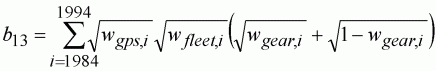 (147)
(147)
Similarly the result for the cell representing observations with GPS and the improved gear, irrespective of fleet or age group is:
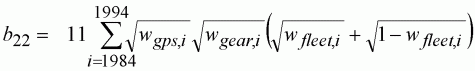 (148)
(148)
and so on. Notice in this case we have 11 observations within each category as we are summing over age groups. The resulting information matrix (Table 10.15) shows a similar pattern to Table 10.14, with most non-diagonal elements remaining at zero.
The observed y-variables are the adjusted log-CPUE. The adjustment is derived from the population model and is a fixed offset when fitting the linear model (i.e. there is no parameter to be fitted to this input). This means either the x or y-variables can be adjusted without affecting the error model, but it is much more efficient to apply the adjustment to the y-variable. The population size is used for the observer survey model and fishing mortality for the total effort model:
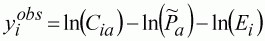 (149)
(149)
where i= observer data grouping (refers to the GPS-gear-fleet/age combination), and
 (150)
(150)
where i= year.
To create the final information matrix, equivalent cells are added:
 (151)
(151)
where la and lb are the relative weights given to observer survey and total effort data models respectively. Similarly, equivalent rows are added in the xy-vector. This final matrix can be decomposed by SVD to obtain the least-squares estimates.
Table 10.15 Information matrix of the weighted dummy variables for the total effort and fishing mortality model. The patterns in the matrix are similar to Table 10.14.
|
|
GPS |
Gear |
1 |
2 |
3 |
4 |
5 |
6 |
7 |
8 |
9 |
10 |
11 |
1 |
2 |
3 |
4 |
5 |
6 |
7 |
8 |
9 |
10 |
11 |
|
GPS |
35.53 |
19.46 |
1.35 |
1.35 |
1.35 |
1.35 |
1.35 |
1.35 |
1.35 |
1.35 |
1.35 |
1.35 |
1.35 |
1.88 |
1.88 |
1.88 |
1.88 |
1.88 |
1.88 |
1.88 |
1.88 |
1.88 |
1.88 |
1.88 |
|
Gear |
19.46 |
115.43 |
5.23 |
5.23 |
5.23 |
5.23 |
5.23 |
5.23 |
5.23 |
5.23 |
5.23 |
5.23 |
5.23 |
5.26 |
5.26 |
5.26 |
5.26 |
5.26 |
5.26 |
5.26 |
5.26 |
5.26 |
5.26 |
5.26 |
|
1 |
1.35 |
5.23 |
11.91 |
0 |
0 |
0 |
0 |
0 |
0 |
0 |
0 |
0 |
0 |
0 |
0 |
0 |
0 |
0 |
0 |
0 |
0 |
0 |
0 |
0 |
|
2 |
1.35 |
5.23 |
0 |
11.91 |
0 |
0 |
0 |
0 |
0 |
0 |
0 |
0 |
0 |
0 |
0 |
0 |
0 |
0 |
0 |
0 |
0 |
0 |
0 |
0 |
|
3 |
1.35 |
5.23 |
0 |
0 |
11.91 |
0 |
0 |
0 |
0 |
0 |
0 |
0 |
0 |
0 |
0 |
0 |
0 |
0 |
0 |
0 |
0 |
0 |
0 |
0 |
|
4 |
1.35 |
5.23 |
0 |
0 |
0 |
11.91 |
0 |
0 |
0 |
0 |
0 |
0 |
0 |
0 |
0 |
0 |
0 |
0 |
0 |
0 |
0 |
0 |
0 |
0 |
|
5 |
1.35 |
5.23 |
0 |
0 |
0 |
0 |
11.91 |
0 |
0 |
0 |
0 |
0 |
0 |
0 |
0 |
0 |
0 |
0 |
0 |
0 |
0 |
0 |
0 |
0 |
|
6 |
1.35 |
5.23 |
0 |
0 |
0 |
0 |
0 |
11.91 |
0 |
0 |
0 |
0 |
0 |
0 |
0 |
0 |
0 |
0 |
0 |
0 |
0 |
0 |
0 |
0 |
|
7 |
1.35 |
5.23 |
0 |
0 |
0 |
0 |
0 |
0 |
11.91 |
0 |
0 |
0 |
0 |
0 |
0 |
0 |
0 |
0 |
0 |
0 |
0 |
0 |
0 |
0 |
|
8 |
1.35 |
5.23 |
0 |
0 |
0 |
0 |
0 |
0 |
0 |
11.91 |
0 |
0 |
0 |
0 |
0 |
0 |
0 |
0 |
0 |
0 |
0 |
0 |
0 |
0 |
|
9 |
1.35 |
5.23 |
0 |
0 |
0 |
0 |
0 |
0 |
0 |
0 |
11.91 |
0 |
0 |
0 |
0 |
0 |
0 |
0 |
0 |
0 |
0 |
0 |
0 |
0 |
|
10 |
1.35 |
5.23 |
0 |
0 |
0 |
0 |
0 |
0 |
0 |
0 |
0 |
11.91 |
0 |
0 |
0 |
0 |
0 |
0 |
0 |
0 |
0 |
0 |
0 |
0 |
|
11 |
1.35 |
5.23 |
0 |
0 |
0 |
0 |
0 |
0 |
0 |
0 |
0 |
0 |
11.91 |
0 |
0 |
0 |
0 |
0 |
0 |
0 |
0 |
0 |
0 |
0 |
|
1 |
1.88 |
5.26 |
0 |
0 |
0 |
0 |
0 |
0 |
0 |
0 |
0 |
0 |
0 |
10.65 |
0 |
0 |
0 |
0 |
0 |
0 |
0 |
0 |
0 |
0 |
|
2 |
1.88 |
5.26 |
0 |
0 |
0 |
0 |
0 |
0 |
0 |
0 |
0 |
0 |
0 |
0 |
10.65 |
0 |
0 |
0 |
0 |
0 |
0 |
0 |
0 |
0 |
|
3 |
1.88 |
5.26 |
0 |
0 |
0 |
0 |
0 |
0 |
0 |
0 |
0 |
0 |
0 |
0 |
0 |
10.65 |
0 |
0 |
0 |
0 |
0 |
0 |
0 |
0 |
|
4 |
1.88 |
5.26 |
0 |
0 |
0 |
0 |
0 |
0 |
0 |
0 |
0 |
0 |
0 |
0 |
0 |
0 |
10.65 |
0 |
0 |
0 |
0 |
0 |
0 |
0 |
|
5 |
1.88 |
5.26 |
0 |
0 |
0 |
0 |
0 |
0 |
0 |
0 |
0 |
0 |
0 |
0 |
0 |
0 |
0 |
10.65 |
0 |
0 |
0 |
0 |
0 |
0 |
|
6 |
1.88 |
5.26 |
0 |
0 |
0 |
0 |
0 |
0 |
0 |
0 |
0 |
0 |
0 |
0 |
0 |
0 |
0 |
0 |
10.65 |
0 |
0 |
0 |
0 |
0 |
|
7 |
1.88 |
5.26 |
0 |
0 |
0 |
0 |
0 |
0 |
0 |
0 |
0 |
0 |
0 |
0 |
0 |
0 |
0 |
0 |
0 |
10.65 |
0 |
0 |
0 |
0 |
|
8 |
1.88 |
5.26 |
0 |
0 |
0 |
0 |
0 |
0 |
0 |
0 |
0 |
0 |
0 |
0 |
0 |
0 |
0 |
0 |
0 |
0 |
10.65 |
0 |
0 |
0 |
|
9 |
1.88 |
5.26 |
0 |
0 |
0 |
0 |
0 |
0 |
0 |
0 |
0 |
0 |
0 |
0 |
0 |
0 |
0 |
0 |
0 |
0 |
0 |
10.65 |
0 |
0 |
|
10 |
1.88 |
5.26 |
0 |
0 |
0 |
0 |
0 |
0 |
0 |
0 |
0 |
0 |
0 |
0 |
0 |
0 |
0 |
0 |
0 |
0 |
0 |
0 |
10.65 |
0 |
|
11 |
1.88 |
5.26 |
0 |
0 |
0 |
0 |
0 |
0 |
0 |
0 |
0 |
0 |
0 |
0 |
0 |
0 |
0 |
0 |
0 |
0 |
0 |
0 |
0 |
10.65 |
10.5.1.4 Results
In an Excel spreadsheet, the model takes about half the time to fit using a non-linear solver if the linear component is fitted separately. However, you will need to set up the model in a form, which avoids inefficiencies in the way the spreadsheet is calculated.
We can see how well the model performs by plotting the residuals. The observer survey data indicates some problems with decreasing variation with larger expected values (Figure 10.2). This is often due to taking logarithms of data, where the variance increases less dramatically than expected with the mean. A second problem with logarithms is that they do not cope with zero values. To get around this a constant was added to all values before taking logs. The constant cannot be estimated. The current value, 1.0, was chosen to minimise the effect of negative residual outliers. The errors are not so badly modelled that we would reject the results, although there is room for improvement. There are alternative approaches to dealing with errors in generalised linear models, which allow multiplicative models, but use variance functions instead of transforms. The cost is increasing the number of iterations to find a solution.
Figure 10.2 Residuals plotted against expected values for the observer survey model. The residuals suggest a decreasing variance with larger expected values. This suggests that there is room for improvement in the error model.
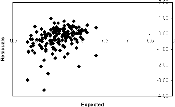
Figure 10.3 Observed and expected log-effort based on the fitted model. The model exhibits systematic error in the time series. The effort is overestimated in recent years suggesting that catchability is underestimated. This would be of great concern in recommending future effort levels. The systematic trend can be reduced by weighting in favour of the total effort model against the observer survey model, at a cost of a poorer fit to the observer survey. However, if the effort data is poor, it may be felt it is more likely trends like this is due to poor data than the fitting process.
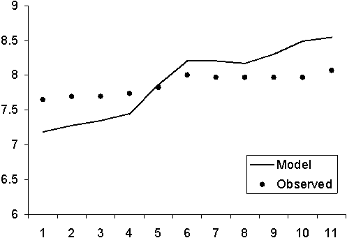
A common problem in combining separate data sets is that error models are incompatible. The main tool for improving compatibility is to weight data appropriately. Firstly, we might introduce a weighting scheme in the observer survey model to account for the increasing variance for smaller expected CPUE. Secondly, we might increase the weight on the total effort series, forcing the estimated effort to follow the observed effort more closely. In most cases, we would probably only have a vague idea of the relative variance of the two series, so this decision would probably be mostly down to judgement. As the weight for the total effort model is increased, it would be necessary to check whether the effect was primarily on catchability or fishing mortality, and what implication the weighting scheme would have on decision-making.
Although we may have estimated the current population sizes and catchability parameters as well as possible, we still need to interpret the results and provide a summary of the stock status. We achieve this by calculating some indicators of stock status, together with their reference points.
Reference points are required for the interpretation of indicators. For example, an indicator might be the spawning stock biomass (SSB). However, if the SSB was reported as 120 000 tonnes, without a reference point it is not possible to know whether this indicates an overfished stock.
The unexploited spawners per recruit can be calculated by using the spawning ratio in each age group and natural mortality. For this, we need an estimate of the proportion surviving to each age in the unexploited stock:
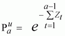 (152)
(152)
or recursively as:
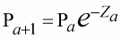 (153)
(153)
where Za is the total mortality at age and is equivalent to natural mortality in the unexploited stock:
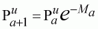 (154)
(154)
If spawning, for example, occurs during the year, rather than on the 1st January, the estimates can be adjusted to represent the survivors to this time:
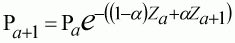 (155)
(155)
where a is the proportion of the year which passes before spawning occurs. The expected survivors gives us a range of per recruit reference points and indicators. We can sum the product of survivors multiplied by some attribute such as weight of the fish (biomass) or proportion mature (spawners) or fecundity (eggs):
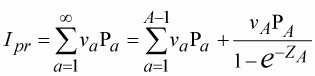 (156)
(156)
where va is the average weight, proportion mature, egg production etc. at age a, and A is the plus group of the population. A reference point is any value that Ipr can become and which can usefully be compared to the current value. Zero is always an implicit reference point, but by-itself is of little value. To scale Ipr we also need to know its maximum value, which will occur when there is no fishing (Equation 154). The ratio of the current indicator value to its maximum gives a dimensionless indicator as a percentage of the stock status with respect the attribute va.
Using Equation 156, the total spawning stock biomass (SSB) can be calculated and compared with an unexploited stock. In this case, however, we need to include some model of recruitment. Again, we chose a simple model, the arithmetic mean of the observed recruitment series (although the median value could just as easily have be chosen if the recruitment estimates were very widely dispersed).
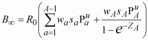 (157)
(157)
where wa is the weight at age, sA is the proportion spawning at age and R0 is the mean number of recruits. The current SSB is the current estimates of the population size at age multiplied by their average weight.
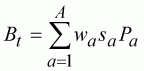 (158)
(158)
Again the ratio Bt/B¥ is a useful reference point to measure how far below the unexploited SSB the current population is. Note that it is possible, although unlikely, that the current SSB lies above the unexploited level if the exploitation rate is low and there have been a series of recruitments greater than the average in the recent past.
The biomass level is a snap-shot of the current population size. These snap shots can be taken forward in time as long as any external variables, such as effort and recruitment are known. The projections use the same models as described in the estimation procedure with the best estimates from the least-squares fit. The recruitment in both years is assumed to be the mean of the estimated recruitment series, and the effort and fleet is assumed to remain constant with the exception that the proportion of vessels using GPS increases to around 75% from 55%. This proportional change in GPS use is applied to the 1994 fishing mortality which otherwise remains the same.
Reference points have an important role in minimising the effect of unknown factors which otherwise have a dramatic effect on uncertainty. References to the unexploited stock primarily aim to remove the effect of natural mortality. Varying natural mortality over the whole life history mostly rescales the stock size rather than affects the fitted model. Although small changes can have very large effects, by using reference points we largely eliminate them. However, if natural mortality changes within the life history, while reference points help reduce these effects, they do not eliminate them altogether and this source of uncertainty may need to be addressed more directly.
10.6.1 Specifying Errors
10.6.2 Results
Bootstrapping is a very powerful technique to explore the effect of random errors on the estimation technique. Bootstrapping is also used in medium-term simulations, Section 9.4, and for calculation of confidence intervals on parameters and reference points, Section 7.3. Bootstrapping is based on Monte Carlo techniques used to generate simulated datasets with known error properties. To demonstrate the approach, we use the analysis described above, including the observer survey and total effort link models.
The aim of bootstrapping methods is to simulate data sets with errors to test how well the estimation procedure works. The data sets should be simulated, as nearly as possible, to exactly the same form as the original data in the fit. Least-squares estimates produce fitted values (expected values) and residuals. By randomising or simulating the residuals, we can produce new imaginary data sets to which the estimation procedure can be applied.
Although we do not do it here, the procedure can easily be extended to deal with all sources of uncertainty:
Fixed Parameters: Some parameters are given as fixed known values when in reality they are poorly known, such as natural mortality. While use of reference points deals with natural mortality as a scaling factor, the other effects of the particular choice of value are unknown. The simplest way to explore this issue is to simulate the error in the parameter and see how it affects the final estimated statistics.
Structural Errors: The fitted model is often called the estimation model. However, biologists may possess alternative more complex models describing the population dynamics in a way that they feel is closer to reality. While the type of data available may prevent fitting these models, they may still be used to simulate data. This allows the analyst to assess the effect of possible structural errors in the estimation model.
Management Controls: It is also possible to simulate the whole management process. This procedure requires not only simulated data, but also management controls, which are applied when particular results are returned from the stock assessment. By projecting the fishery forward, we can see how well the rules perform when knowledge is less than perfect. This should be the ultimate arbiter on both the assessment advice and management controls.
We only consider estimating the variation of the fitted parameters, the basic Monte Carlo simulation. Extensions to this would allow all the types of simulations above. However, the principles remain the same (see Figure 10.4). The simulations provide a frequency framework to describing uncertainty and its implications to management.
Figure 10.4 The general bootstrap procedure for investigating the performance of estimation methods. Although all procedures are broadly the same, they may be based on different sources for the random variables. The bootstrap approach can be used to estimate the degree of bias, the parameter confidence intervals or any other issue related to uncertainty.
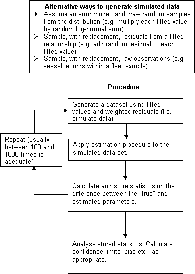
We are simulating the estimation model only. The original data in the model were the scientific survey population indices, the observer vessel survey and the total effort. Catches were assumed to be known exactly, so they have no error.
Errors for the population index and observer survey can be derived in the same way. The original data is decomposed into the least-squares fitted value for the data point, and the residual, the difference between the observed and fitted value. It is the sum-of-squares of the residuals that the model fitting process aims to minimise. These residuals can be randomly sampled-with-replacement and added to the fitted value to create a new data set. For the population survey data this is straightforward. For the observer survey we can only simulate the transformed variable (Ln(Yi+1)). This means that some simulated values cannot be translated back to real catches (i.e. when the simulated value is less than one), which is a direct artefact of the presence of zeros in the data. Although not entirely satisfactory, it is unlikely that the few values for which this is a problem will influence the results of the simulation too greatly.
Although we can generate fitted values and residuals for the log total effort series, there are only 11 data points. A fundamental assumption of bootstrapping is that each set of random residuals and hence simulated data, is random and independent. While for non-parametric bootstraps this is always violated, the dependence effect is small for large data sets. In these circumstances, the robustness of not having to specify any particular error distribution more than out-weighs this cost in accuracy. For small data sets, the use of residuals is moot. For these the correlation between simulated data sets would probably mean the variation in fitted parameters is biased or underestimated. Under these circumstances, it is better to simulate the error from a parametric probability distribution, but make the simulated error similar to the observed residuals. Hence, for the current analysis we could simulate normal errors based on the standard deviation of the residuals. These could be added to the fitted effort values in exactly the same way to create new simulated effort data, except that we would convert residuals with a clear pattern (Figure 10.3) to a series with random errors and no pattern.
So far we have assumed that the errors are well-behaved. That is the errors within each model are independent identically distributed random variables. In many cases they are not, but we would still like to construct an error simulation. If weights vary between data records the method is straightforward. The weights are the inverse (relative) variance, so we can standardise all the residuals by multiplying them by the square root of the weight (often called the Pearson residual). These standardised residuals can be sampled and divided by the appropriate weight before adding to the fitted value.
Suspected systematic error (e.g. Figure 10.3) is more difficult to deal with. Effectively we need to propose a second model. Systematic errors often occur in time series and may take the form of autocorrelation or trends. If autocorrelated, you may wish to weight the model in line with the level of autocorrelation as the series effectively contains less information than might at first appear. This takes the form of weighting the series (in addition to other weights) by a factor related to the autocorrelation. This is not necessary if the only data you have is autocorrelated and you plan only to estimate parameter errors through a bootstrap, which is taking account of autocorrelation. However, for relative weights between different data sources this may be a good basis for l. Autocorrelation can be simulated, but we need to define how it has arisen. In most cases, an autoregressive model would probably suffice.
Trends in residuals can be accounted for by linear regression, but a better approach is probably differencing the data. Single differencing removes linear trends, differencing twice removes quadratic trends and so on with higher order polynomials. If, after differencing and applying weights so that the series is stationary, the errors are autocorrelated, some model for the autocorrelation can also be fitted. This then would form the basis for simulation, developing autocorrelated errors from the model and applying a reverse of the differencing to generate random errors which possess the same systematic patterns as those observed from the model fit. If you are familiar with time series analysis, you will by now have noticed a description of Box-Jenkins ARIMA models (Chatfield 1984, Diggle 1990).
The ARIMA approach should only be carried out for the simulation if you have been unable to remove the systematic error in the original analysis. Autocorrelations and residual trends are not desirable, and should, if you simulate the error correctly, increase the uncertainty in the results. However, if they are present, they need to be represented in some way in the simulation so that the full uncertainty is represented and the results are not viewed with misplaced optimism. If, on completing the simulations, the stock status and recommendations are, overall, not affected by this source of error, recommendations can still be made despite misgivings about the final form of the model.
Figure 10.5 Original (- -) and simulated (--) residuals for the log-total effort model. The systematic trend is maintained, but the simulated residuals show random divergence from the original systematic trend. The simulated data represent data that we could have obtained if the underlying model is correct, but that the errors are influenced by time series effects that are unaccounted for.
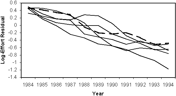
So, we certainly have misgivings about the total effort model (Figure 10.35). Assuming that we are unable to fix the problem in the original model in the time available, how should we represent it in the simulation. We firstly obtain the residuals in the normal way. They have a negative slope. The first differences have no slope, and no obvious autocorrelation (the time series is short, however). If we assume the slope is systematic as opposed to random, we can use the fixed mean of the differences to represent the trend. So, we simulate the error as a normal variate with mean and standard deviation equal to the mean and standard deviation of the differences. It should be emphasised this does not solve the problem in sense that the unknown bias continues to be present, but at least you can simulate realistic data sets that include the residual trend.
Once the simulated data are obtained the full model is fitted to those data in exactly the same way as in the original least-squares model to obtain simulated parameter estimates, indicators and reference points. These can be stored in a table for analysis.
Overall the fit and subsequent bootstrap estimates relate well to the underlying “true values” used to simulate the original data (Table 10.15). In particular, it is worth checking the parameter bias, as these can be very large in some cases so that the true value lies outside the confidence intervals. Bias while present, is not so large as to invalidate the results and broadly they are correct. The stock is overfished and the situation will only get worse unless urgent action is taken.
The exception, and a very important one, is the recruitment in 1994. Despite the simulation the variation estimated in this parameter is small and the true value lies well outside the confidence region. While it is easy to understand why the estimate is relatively poor (there is less data relevant to its estimation), but why is the confidence interval so narrow. This is an artefact of the bootstrap. In order to improve the fitting time, we start the parameters from their least-squares values. The non-linear optimiser will carry on moving parameters around as long as there is significant improvement in the objective function. If the parameter is having too small an effect, the parameter will not be moved (by default). Hence, a parameter may take on similar consecutive values because the likelihood surface with respect to the parameter is very flat. So, it has very little effect on the sum-of-squares even if it is moved some distance. Because the non-linear optimiser concentrates on the local behaviour of the parameter, it gives up moving it although it may be a long way from its maximum point. While this is not necessarily a problem in the sense that the maximum point is probably not much of a better estimate than the current point, it does suggest in simulations that the parameter is much more accurate than it really is. This problem needs to be guarded against. One option is to increase the precision of the optimiser. Unfortunately, this is will greatly slow up the fitting process and does not guarantee success. A second is to try different starting points either between simulated data sets or for the same data set. This is preferable, but the software managing the bootstrap will need to be more sophisticated as the fitting process is much more likely to hit problems requiring intervention.
Table 10.15 Results from fitting the model to simulated data, including bootstrap average and 90% confidence interval from 500 simulations. Perusal of the table indicates that the model fit performed well overall, and that the stock is heavily overfished. As can be seen from the “true values”, used to simulate the real data, this is the correct interpretation. Where there are biases, they are correctly identified by the bootstrap. This general result is no surprise as the structural errors are minimal (i.e. the model used to simulate the data was largely the same as that to fit the model).
|
Year 1994 |
1 |
2 |
3 |
4 |
5 |
6 |
7 |
8 |
9 |
10 |
|
|
True Values |
461026 |
103220 |
85468 |
16110 |
2655 |
5602 |
2900 |
1165 |
407 |
116 |
|
|
Least-Squares |
517903 |
106974 |
93494 |
16161 |
2831 |
5972 |
3044 |
1303 |
560 |
230 |
|
|
Average |
518083 |
105438 |
97466 |
17305 |
3027 |
6644 |
3311 |
1440 |
597 |
223 |
|
|
0.05 |
516218 |
90626 |
84678 |
15456 |
2546 |
5746 |
2779 |
1199 |
489 |
181 |
|
|
0.95 |
520313 |
118067 |
115511 |
19853 |
3604 |
7830 |
3888 |
1718 |
726 |
272 |
|
|
Age 10 |
1984 |
1985 |
1986 |
1987 |
1988 |
1989 |
1990 |
1991 |
1992 |
1993 |
1984, 11 |
|
True Values |
1618 |
2374 |
2810 |
4145 |
5496 |
4806 |
4301 |
1293 |
929 |
515 |
1507 |
|
Least-Squares |
892 |
1137 |
1866 |
3491 |
6141 |
5654 |
4154 |
1645 |
1073 |
602 |
386 |
|
Average |
650 |
971 |
1712 |
3136 |
6018 |
5734 |
4169 |
1795 |
1113 |
638 |
222 |
|
0.05 |
553 |
870 |
1559 |
2902 |
5737 |
5510 |
3981 |
1669 |
1051 |
585 |
172 |
|
0.95 |
765 |
1099 |
1903 |
3406 |
6299 |
5993 |
4344 |
1904 |
1177 |
687 |
288 |
|
Reference Points |
S1994 |
S% |
Bunexp |
B1994 |
B1995 |
|
|
|
|
|
|
|
True Values |
0.158 |
0.099 |
1991735 |
48747 |
30059 |
|
|
|
|
|
|
|
Least-Squares |
0.182 |
0.114 |
2079070 |
57994 |
31435 |
|
|
|
|
|
|
|
Average |
0.183 |
0.115 |
2080709 |
63877 |
43365 |
|
|
|
|
|
|
|
0.05 |
0.172 |
0.108 |
2070741 |
55964 |
36179 |
|
|
|
|
|
|
|
0.95 |
0.194 |
0.122 |
2104842 |
75664 |
53947 |
|
|
|
|
|
|
There were other errors introduced, most notably the proportional use of GPS and monofilament gears assumed by the analysis was not true in the simulated data. These and other sources of uncertainty should ideally be included in the simulations. These would widen the confidence intervals, which would then include the true values.
![]()
![]()
![]()