![]()
![]()
![]()
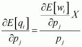
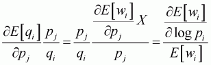
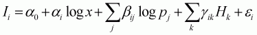
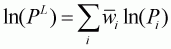
Application of the theory of the household requires a specific model. In general, econometric studies of demand include both single equations and systems of demand equations. The demand functions can be generalized for a consumer or a household buying n goods as:
qi = qi (p1, p2,
... pj, ... pn, I), i = 1, 2, ..., n.
(3.1)
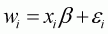
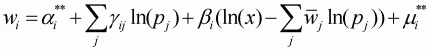
where qi is the quantity demanded; p is the price, the subscript i denotes the commodities; and I is income. These "n equations" can be estimated by single equations or by systems of equations. In this study, Equation 3.1 is estimated in a budget share form. Extending the demand function for individual consumers to that for a group of consumers in most empirical applications requires the inclusion of demographic variables besides prices and income. In this section, the econometric models for 11 food items are described. The same methodology also applies to the model for seven meats.
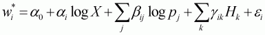
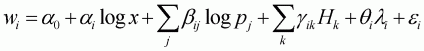
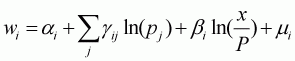
The first empirical model applied in this study is the Working-Leser model. The original form of the Working-Leser model was discussed by Working (1943) and Leser (1963). Intriligator, Bodkin and Hsiao (1996) and Deaton and Muellbauer (1980a) provide a more detailed discussion of this functional form. In the Working-Leser model, each share of the food item is simply a linear function of the log of prices and of the total expenditure on all the food items under consideration. The Working-Leser food demand function can be expressed as:
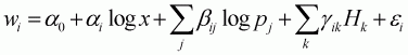
(3.2)
where (i,j) represents the 11 food items; wi is the expenditure share of food i among the 11 food items; pj is the price of food j; and x is the total expenditure of all food items included in the model.
Hk includes dummy variables where k is 25:
AGE = log age of household head;
SIZE = log of household size;
WE = number of wage earners;
BABY = number of children aged five years or under;
PRIM = number of children aged between 6 and 12 years;
HIGH = number of children aged between 13 and 18 years;
M = dummy variables for month (M1, ..., M10);[5]
REG = dummy variables for region (REG1, ..., REG9).
ei's are random disturbances assumed with zero mean and constant variance. This model can be estimated for each food item by the ordinary least squares (OLS).
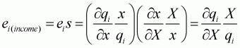
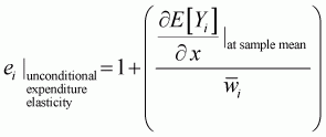
It is easy to show the elasticity formulae for the Working-Leser model. The expenditure elasticity (ei) can be expressed as:
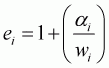 .
.
(3.3)
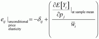
Taking a derivative of Equation 3.2 with respect to log(pj) yields, uncompensated own (j =i) and cross (j ¹i) price elasticities (eij) are as follows:
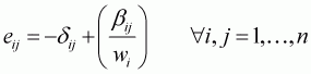
(3.4)
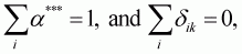
where  is
the Kronecker delta that is unity if i = j and zero otherwise. In this
study, expenditure, own-price and cross-price elasticities are evaluated at
sample means.
is
the Kronecker delta that is unity if i = j and zero otherwise. In this
study, expenditure, own-price and cross-price elasticities are evaluated at
sample means.
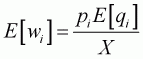
Since the Working-Leser model uses total expenditures for the group of food items included in the model, it does not provide a direct estimate of income elasticity. In order to estimate income elasticity, the following Engel function is estimated:
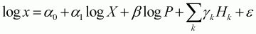
(3.5)
where x is total expenditures of the food included in
the model; X is total expenditures of food and non-food consumer goods and
services; P is Laspeyres price index for the eleven foods; and other demographic
and dummy variables are the same as previously defined. Remaining variables are
the same as those in Equation 3.2. Income elasticity can be estimated from
Equations 3.2 and 3.5. From Equation 3.2, the expenditure elasticity,
 , can be estimated. From
Equation 3.5, the responsiveness of expenditure on food items by income change,
, can be estimated. From
Equation 3.5, the responsiveness of expenditure on food items by income change,
 , can be derived. Hence,
income elasticity is estimated as follows:
, can be derived. Hence,
income elasticity is estimated as follows:
 .
.
(3.6)
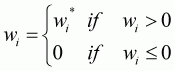
When estimating income elasticities, the use of household-level microdata is a good way of avoiding the aggregation problem. However, the use of household microdata on detailed commodities is comlicated by the econometric problem, which arises when some households have zero consumption of one or more of the items considered. In the FIES, the zero consumption problem is particularly severe for rice, oil and fats and FAFH, among the 11 major food commodities, and for ground meat and bacon, in the seven meats model.
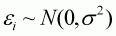
It is known that estimates of coefficients are inconsistent when only observed positive purchase data are used to estimate consumption behaviour by OLS regression. The dependent variables - the budget shares of the food items specified - are zero if a household does not purchase the food item, and positive if it does. Zero shares are censored by an unobservable latent variable. In this report, two different models have been applied to correct zero consumption: Heckman's two-step model and the standard Tobit estimator. The derivation of elasticity measure for each model is shown. Each model is based on different assumptions regarding zero consumption. Zero consumption is observed when no purchase of the particular item was made during the month-long survey period. If zero consumption is assumed to be due to sample selection, Heckman's two-step is the appropriate model. The Tobit model simply captures the corner solutions for utility maximization. The results from the three estimators, including OLS, are compared in the following subsections.
The Tobit estimator and elasticity calculation have been the subject of many studies. Notation follows mainly Amemiya (1985) and Maddala (1983).
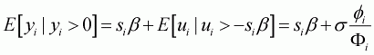
The Tobit estimator is defined as follows:
(3.7)
where b is a k × 1 vector of unknown parameters; si is a k × 1 vector of known variables; ui are residuals that are independently and normally distributed, with mean zero and a common variance s2; and y* is an unobservable latent variable.
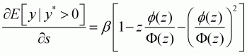
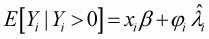
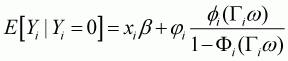
McDonald and Moffitt (1980) describe how total change in y can be disaggregated into two parts: the change in y above the threshold, weighted by the probability of being above the threshold; and the change in the probability of being above the threshold, weighted by the expected value of y. Unconditional elasticity describes the elasticity of y from the mean of all observed values for y. Conditional elasticity is the elasticity measure that is conditional on the consumer's choice to purchase a non-zero quantity of the good.
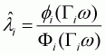
Considering the model given in Equation 3.7 and the non-zero observations yi, the result is:
(3.8)
where fi and Fi are the density function and cumulative
distribution function of the standard normal evaluated at
 . For notational
convenience, z is defined as
. For notational
convenience, z is defined as
 .
.
The following formula is used to obtain predicted values using all the observations:
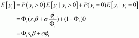
(3.9)
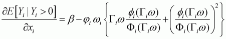
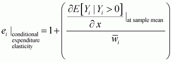
Unconditional and conditional elasticities for a particular variable, s, in a general form can be obtained as follows:
Unconditional elasticity:
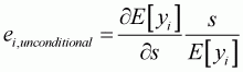
(3.10)
Conditional elasticity:
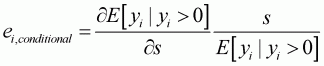
(3.11)
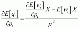
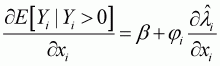
The prediction of yi, given si, can be obtained from the different expectation functions: unconditional and conditional expectations. Following Maddala (1983) and McDonald and Moffitt (1980), unconditional expectation can be obtained from the derivative of Equation 3.9 without the subscript i, which denotes observation:
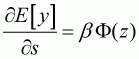
(3.12)
From Equation 3.12, the partial derivative can be calculated as:
(3.13)
(See McDonald and Moffitt [1980] for the detailed derivation.)
From these general formulae for elasticity estimation, the elasticity formulae for the Leser-Working model can be derived. In this study, the Working-Leser Model is denoted as:

(3.14)
 and
and
where subscript i denotes a good in question; X
denotes total expenditure on 11 commodities; pi and
qi denote price and quantity for ith commodity,
respectively; and wi denotes the budget share of ith
good,  .
.
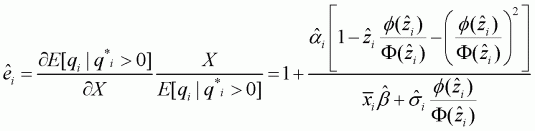
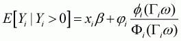
Expenditure elasticity is obtained in the following way:
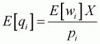
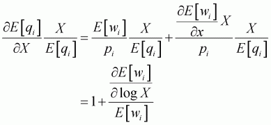
(3.15)
Since the numerator of Equation 3.15 is the coefficient of
Equation 3.14, this formula can be applied to Equation 3.14 evaluated at the
sample mean such that f and F are the density function and cumulative density
function, respectively, of the standard normal evaluated at zi. For
convenience, Equation 3.14 can be rewritten in the compact form:
 .
.
Hence, unconditional expenditure elasticity is:
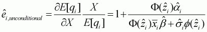
(3.16)
where the upper bar denotes the sample mean, and
 .
.
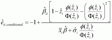
Conditional expenditure elasticity is:
(3.17)
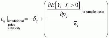
Own-price elasticity becomes:
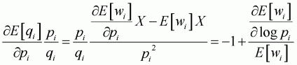
(3.18)
Unconditional own-price elasticity is:
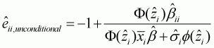
(3.19)
Conditional own-price elasticity is:
(3.20)
In the same format, cross-price elasticity can be obtained as follows:
(3.21)
Unconditional cross-price elasticity is:
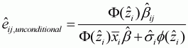
(3.22)
Conditional own-price elasticity is:
(3.23)
In order to correct for the sample bias problem in rice consumption, Heckman's two-step estimation (Heckit) procedure can be applied, as suggested by Heckman (1978). In the first stage, a probit regression is computed in order to estimate the probability that a given household consumes the food item in question. This regression is used to estimate the inverse Mills ratio (l) for each household, which is used as an instrument in the second regression. In the second stage, the initial Working-Leser model (Equation 3.2) with the inverse Mills ratio is estimated.
In the first stage, the household's decision is modelled as a dichotomous choice problem:
(3.24)
where Ii is one if a household consumes ith food item (i.e. wi > 0), and zero otherwise. Other variables have already been defined. From Equation 3.24, the inverse Mills ratio (l) for every household can be computed as:
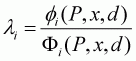
(3.25)
where P, x, d are the vector of prices; expenditures and the vector of demographic variables for the household, respectively; fi is the density probability function; and Fi is the cumulative probability function. For notational convenience, this is set as:
(3.25')
where Gi is a vector
of regressors explaining the binary choice in the first stage; and
 is the conformable
parameter vector.
is the conformable
parameter vector.
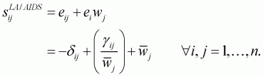
In the second step, the following Working-Leser demand
function incorporating the computed inverse Mills ratio,
 , as an instrument variable
is estimated:
, as an instrument variable
is estimated:
(3.26)
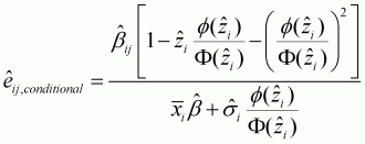
where qi is the parameter associated with the inverse Mills ratio. It is important that only the non-zero observations on wi are used in the second-stage estimation in order to estimate the conditional elasticity.[6] The whole sample is used to estimate the unconditional elasticity.
It is important to note that at least one of the explanatory variables in the first equation is not included at the second step for identification, according to Maddala (1983) Amemiya (1985) and Johnston and DiNardo (1997). The city size dummy variables based on the population are added in the first step: cities are divided into major cities (population of at least 1 million), middle-sized cities (population of 150 000 to 1 million), small cities A (population of 50 000 to 150 000) and small cities B (population of fewer than 50 000).
Even though Heckman's two-step estimator is fairly common in empirical studies, there is little literature on its elasticity estimation. Byrne, Capps and Saha (1996) explicitly show elasticity estimates of Heckman's two-step estimator for a single equation case. Later, Saha, Capps and Byrne (1997) generalized the method from a single equation to a system of equations. For this report, the methodology developed by Byrne, Capps and Saha (1996) and Saha, Capps and Byrne (1997) was adapted and applied to the Working-Leser model.
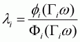
At the first stage, the inverse Mills ratio is estimated by
the dichotomous-choice probit model. In a general form, the estimated inverse
Mills ratio,  , is described
in Equation 3.25. In the second stage equation, the conditional expectation of
the dependent variable can be calculated in a general form as follows:
, is described
in Equation 3.25. In the second stage equation, the conditional expectation of
the dependent variable can be calculated in a general form as follows:
 and
and
(3.27)
where  is
the vector of regressors explaining the magnitude of
is
the vector of regressors explaining the magnitude of
 in the second stage
equation;
in the second stage
equation;  is the associated
parameter vector; and
is the associated
parameter vector; and  is a
parameter corresponding to the estimated inverse Mills ratio, which is estimated
at the first stage. In order to derive conditional elasticity, only the non-zero
observation of is used for
the second stage of Heckman's two-step estimator.
is a
parameter corresponding to the estimated inverse Mills ratio, which is estimated
at the first stage. In order to derive conditional elasticity, only the non-zero
observation of is used for
the second stage of Heckman's two-step estimator.
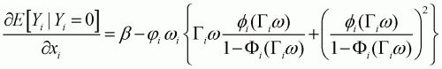
Taking a partial derivative with respect to
( may be considered as any
variable in the vector of regressors):
(3.28)
According to Saha, Cappas and Byrne (1997), this can be simplified as:
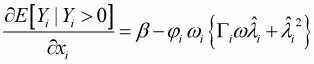
(3.29)
where  and
and
 are parameters
corresponding to and the
inverse Mills ratio at the second stage equation, respectively;
are parameters
corresponding to and the
inverse Mills ratio at the second stage equation, respectively;
 is a parameter associated
with at the first stage;
is a parameter associated
with at the first stage;
 is the vector of regressors
explaining the binary choice in the first stage; and
is the comfortable
parameter vector, as already defined. Marginal effects are evaluated at the
sample mean. The average of the inverse Mills ratio can be estimated by adding
up the results of all the observations and dividing by the number of
observations.
is the vector of regressors
explaining the binary choice in the first stage; and
is the comfortable
parameter vector, as already defined. Marginal effects are evaluated at the
sample mean. The average of the inverse Mills ratio can be estimated by adding
up the results of all the observations and dividing by the number of
observations.
In order to estimate unconditional elasticity, the whole sample needs to be used for the second stage so that zero-consumption households are taken into account. In the second stage estimation, the expectation of the dependent variables becomes as follows:
(3.30)
(3.31)
A partial derivative with respect to
can be taken to produce the
following:
(3.32)
(3.33)
Denoting  as the proportion of observations for which
 , hence
 , Saha. Capps and Byrne
(1997) suggest taking a weighted average of these two biases, as
follows:
, Saha. Capps and Byrne
(1997) suggest taking a weighted average of these two biases, as
follows:
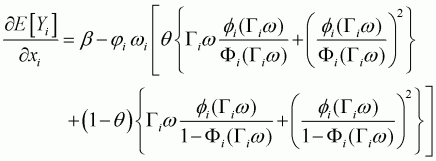
(3.34)
The sample mean for the bias term is calculated as before: the bias terms of each observation are added together and the result is divided by the number of observations.
In order to apply these computations for the Working-Leser model, the marginal value needs to be adjusted to follow the elasticity formula. It then becomes possible to calculate the elasticities for conditional price, conditional expenditure, unconditional price and unconditional expenditure, as follows:
(3.35)
(3.36)
(3.37)
(3.38)
Deaton and Muellbauer (1980a; 1980b) developed a flexible demand system called the "almost ideal demand system" (AIDS). The concept of a flexible demand system is extremely useful for estimating a demand system with many desirable properties. As Moschini (1998) pointed out, the AIDS model automatically satisfies the aggregation restriction, and with simple parametric restrictions, homogeneity and symmetry can be imposed. In addition, the non-linear Engel curves of the AIDS model imply that an increase in income will lead to a decrease in the share of income allocated to a particular commodity, as well as a decrease in the income elasticity of that good when it is less than one. However, the AIDS model may be difficult to estimate because the price index is not linear in terms of parameters estimated. Owing to its simplicity, the linear approximate almost ideal demand system (LA/AIDS) is popular for empirical studies. Both the LA/AIDS and the AIDS models were applied for this report.
The AIDS model for the 11 food commodities can be estimated as follows:
 i = 1, ...,
11
i = 1, ...,
11
(3.41)
where wi is the budget share of good i; pj is the price of good j; x is the total expenditure of the goods in question; mi is the random disturbances assumed with zero mean and constant variance; and P is a translog price index defined by:
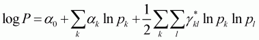
(3.42)
Where k is = 1, ..., 11; l is 1, ..., 11; and the gij parameters are defined under symmetry as follows:
 j = 1, ...,
11
j = 1, ...,
11
(3.43)
The model defined by Equations 3.41 to 3.43 is called the AIDS model.
It is easy to check that the adding-up restriction is
satisfied with the given  for all j:
 ,
,
 , and
, and

(3.44)
The homogeneity restriction is satisfied for the AIDS model if, and only if, for all j:

(3.45)
The symmetry is satisfied by:

(3.46)
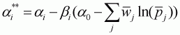
Using the price index in Equation 3.42 raises estimation difficulties caused by the non-linearity of parameters. In addition, the theory of the household does not provide any empirically plausible value for a0.
As Asche and Wessells (1997) point out, the Stone index is widely used for LA/AIDS estimation:
 i = 1,
..., 11
i = 1,
..., 11
(3.47)
where w is budget share among the 11 commodities. The Stone index is an approximation proportional to the translog, i.e. P = j P* where E(ln(j)) = a0. The LA/AIDS model with the Stone index can be denoted as follows:
(3.48)
where
 and
and
 .
.
Since prices will never be perfectly collinear, it is widely
cited that applying the Stone index will introduce the units of measurement
error (see Alston, Foster and Green, 1994; Asche and Wessells, 1997; Moschini,
1995). The Stone index does not satisfy the fundamental property of index
numbers because it is variant to changes in the units of measurement for prices.
One of the solutions to correct the units of measurement error is that prices
are scaled by their sample mean. Following Moschini's suggestion (1995), a
Laspeyres price index can be used to overcome the measurement error.
Specifically, the log-linear analogue of the Laspeyres price index is obtained
by replacing  in Equation
3.47 with
in Equation
3.47 with  , which is a mean
budget share. Hence, the Laspeyres price index becomes a geometrically weighted
average of prices:
, which is a mean
budget share. Hence, the Laspeyres price index becomes a geometrically weighted
average of prices:
(3.49)
Substitution of Equation 3.49 into Equation 3.48 yields a LA/AIDS model with the Laspeyres price index as follows:
(3.50)
where
 .
.
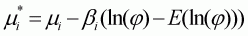
Following Pollak and Wales (1978; 1981), linear demographic
translating is applied,  ,
where d and h are
associated parameters and demographic variables, respectively. In this study,
linear demographic translating replaces Equation 3.41 as follows:
,
where d and h are
associated parameters and demographic variables, respectively. In this study,
linear demographic translating replaces Equation 3.41 as follows:

(3.51)
where  .
The demographic and dummy variables used in the complete demand system are the
same as the ones used in single equation models.
.
The demographic and dummy variables used in the complete demand system are the
same as the ones used in single equation models.
The adding-up restriction requires:
 k = 1,
..., m
k = 1,
..., m
(3.52)
where m is the number of demographic and other dummy variables.
In order to correct for the zero consumption problem, the generalized Amemiya's two-stage estimators are applied to a simultaneous-equation model (see Amemiya, 1974; Lee and Pitt, 1986; and Heien and Wessells, 1990). In the first stage, the probit model with dichotomous choices is estimated. The inverse Mills ratio is derived from the regression results. For the LA/AIDS model, the inverse Mills ratios of only rice, fats and oil and FAFH are used. These three inverse Mills ratios are used as instruments in the second stage. Similar arguments are adopted from the Heckman's two-step estimator, as already discussed.
The elasticity derivations for the AIDS and LA/AIDS models are widely investigated and well documented. Following Buse (1994) and Green and Alston (1990), taking the derivative of Equation 3.48 with respect to ln(x), the expenditure elasticity ei can be obtained as follows:
(3.53)
Taking the derivative with respect to
ln(pj), uncompensated own- (j =i) and cross-
(j ¹i) price elasticities,
 , become as
follows:
, become as
follows:
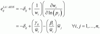
(3.54)
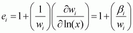
where  is
the Kronecker delta that is unity if i = j, and zero otherwise. In this
study, the sample mean is used for the point of normalization.
is
the Kronecker delta that is unity if i = j, and zero otherwise. In this
study, the sample mean is used for the point of normalization.
The Hicksian compensated price elasticities can be derived for
the AIDS and LA/AIDS models. The compensated price elasticities,
 , at the point of
normalization become as follows:
, at the point of
normalization become as follows:
(3.55)
For the AIDS model, following Buse (1994), Equation 3.53 is
applied for expenditure elasticity. Following Green and Alston (1990),
uncompensated own- and cross-price elasticities,
 , become as
follows:
, become as
follows:
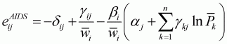 .
.
(3.56)
Compensated own- and cross-price elasticities,
 , become as
follows:
, become as
follows:
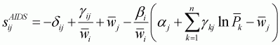 .
.
(3.57)
|
[5] Only ten monthly dummies
are included in the model because CPI data for FAFH are obtained on a monthly
basis. [6] When a system of equations with inverse Mills ratio is used, the convention is to use the whole sample. |
![]()
![]()
![]()