5. RESULTS

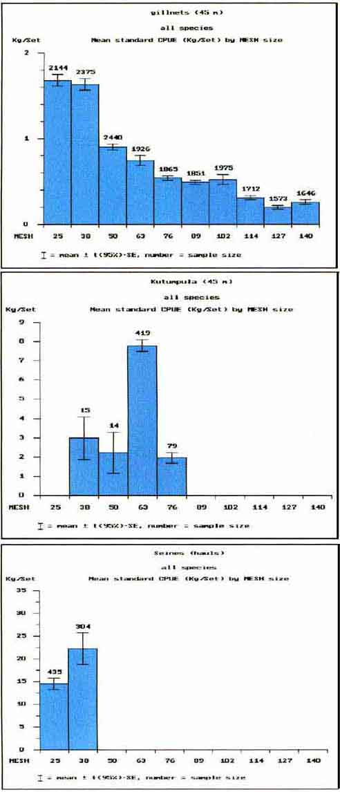
Figures 6a to 6c show the mean catch per unit effort in the different mesh sizes by the three gears sampled in this study. Although a few mesh sizes are missing in the kutumpula and seine samples, it is noticeable how close the CPUE pattern by mesh size follows the frequency distributions of the mesh sizes in the fishery (Table 4). Also the relative abundance of the three gear types in the fishery (Table 4) is in close inverse accordance with the overall catch rates of each type (Figure 6 and Table 12).

FIGURE 6

A. Cpue_(kg) in different mesh sizes for experimental gillnets operated by local fishermen

B. Cpue_(kg) in different mesh sizes for kutumpula nets operated by local fishermen

C. Cpue_(kg) in different mesh sizes for seine nets operated by local fishermen

5.1 Catch composition in different gears

Adistinct difference in catch composition can be observed between the sampling gears (Tables 6 and 7). Furthermore, catches from the GNS by DoF differ to a large extent from the catches realizsed by fishermen using the same gear (experimental gillnets). For example, in the GNS the most important species is Alestes macrophthalmus, both by number as well as by weight, while in the fishers experimental nets this species contributes only marginally (<11 percent by number and one percent by weight) to the catch. This can be attributed to different ways of setting the nets. While the DoF surveys primarily set the nets in the open water patches (a.o to reduce the amount of work in cleaning the nets from weeds), fishermen set the nets closer to the banks to target specific species and to improve their catch rates. The results show that the GNS catches in the swamps are not representative for the species composition in the artisanal gears.

TABLE 6. Relative catch composition, percent number, for the different sampling gears used in this study. Data collected from July 1994 to July 1996, FDC broken down by method. Species contributing with less than 1 percent to the total catch are grouped in “other species”.

TABLE 7. Relative catch composition, percent weight, for the different sampling gears used in this study. Data collected from July 1994 to July 1996, FDC broken down by method. Species contributing with less then one percent to the total catch are grouped in “other species”.

The number of species caught also differs by method. GNS and Lundgren nets show the highest species diversity with 19 and 18 different species contributing more than one percent by weight to the total catch. The fishermen using experimental nets, their own nets, and seines have respectively 15, 14 and 15 different species in their catch, and kutumpula target only eight main species. Thus, the three artisanal methods: gillnets, kutumpula and seines, are targeting different parts of the fish community in the swamps. Gillnets are mainly catching smaller species such as M. macrolepidotus and T. sparmanii, Kutumpula is highly selective on cichlids (96.3 percent by number and 92.0 percent by weight), particularly T. rendalli which is well known for its ability of evading stationary gillnets (e.g. Kenmuir, 1984), and the seines are mainly directed at the Mormyridae (59.3 percent by number and 58.9 percent by weight).

5.2 Estimates of vital parameters and long-term yield predictions

Table 8 gives a summary of estimated vital parameters for the selected species. Total mortality Z from the catch curve analysis and natural mortality M from Pauly’s formula were used to calculate F and E. The table also includes the length-weight coefficients a and b used for estimating weights (e.g. weight infinity). For some of the larger species (H. vittatus, C. gariepinus, O. macrochir, T. rendalli and S. robustus), 2 cm length class intervals were used because FiSATcan only handle up to 50 length groups at a time. Adetailed presentation of the derivation of vital parameters and long term yield predictions for the individual selected species in this study are presented in Kolding, Ticheler and Chanda (1996a, 1966b).

For only one of the selected species in the Bangweulu fishery, Hydrocynus vittatus, reliable growth parameters have been obtained previously from scale readings (Griffith, 1975). These were used to fit a comparative growth curve on the length-frequencies for H. vittatus in this study. The results showed that the two separate estimates produced nearly identical growth curves in the length interval observed, although Griffith had derived an L_¥ that was 20 cm larger. Separate growth parameters for M. macrolepidotus were estimated for experimental gillnet data as well as for data obtained from Lundgren nets. Again the results were comparable over most of the length range, although the Lundgren data yielded a rather low estimate of L_¥. It was therefore decided to continue with the set of estimates obtained from the experimental gillnet data.

For two species the estimates for M were bigger than for Z. This indicates that fishing mortalities for these species were extremely low and consequently the exploitation rates close to zero. The reason that estimates for M can be bigger than Z estimates (when F is very small) should be attributed to noise in the data and because M and Z are independent estimates (Section 2.2.6) from different methods.

TABLE 8. Summary of growth, mortality and length-weight parameters for selected species from length frequency analysis. L_¥, W_¥, and K are the parameters for the von Bertalanffy growth equation, j‘ is the growth performance index (Munro and Pauly, 1983), Z and CI_Z1 is the estimated total annual mortality and the 95 percent confidence intervals. M is the natural annual mortality, F is the annual fishing mortality, E is the exploitation rate (F/Z), a and b are the coefficients for the length-weight regressions.

*second Z estimate for H. vittatus based on growth parameters from Griffith (1975).
^† Growth parameters for S. mellandi were obtained from Kolding, Ticheler and Chanda (1996a).
^‡ Z from the empirical relationship: Z = 13.49 * W_¥ exp(-0.33) (Marshall, 1993).
^§ values from B. paludinosis.

Table 9 (sorted by the size of the species) gives a summary of the long term Thompson and Bell yield predictions for the various species by the three important fishing methods (artisanal stationary gillnets, kutumpula and seines).

TABLE 9. Summary of Thompson and Bell long term yield predictions by species and catch method (single species- single gear), sorted by descending order of the size of the species (L_¥). LM is the observed modal length of the catch. L50 percent catch is the length at which 50 percent or more of the catch is smaller than or equal to this length. F-mean is the mean fishing mortality and E-mean is the mean exploitation rate (the latter two were obtained from the cohort analysis), values of E-mean higher then 0.5. are indicated in bold. The effort-factor is the fraction at which the current fishing pressure should be altered to achieve the long term theoretical Maximum Sustainable Yield (MSY, whereby 1 = present effort; >1 is under - and <1 is overexploitation). The column MSY-Yield gives the absolute changes between Present Yield and long term MSY if the effort factor was applied. The last column ranks the species-gear combinations on present yield contributing more than 10 tonnes per year with the three largest are highlighted.

Table 9 shows that in terms of present yield in the Bangweulu swamps, the three dominant species are:

• the small Marcusenius macrolepidotus (which is caught in the large quantity of some 700 tonnes per year in both seines and small meshed gillnets),

• the medium sized Tilapia rendalli (420 tonnes in kutumpula), and

• the small Tilapia sparmanii making up around 260 tonnes in the gillnets.

Each of the three different gears occupies one of the first three ranks according to yield. The next five ranks, yielding between 135 to 100 tonnes per year, consist of the large Clarias gariepinus (gillnets) and the three relatively large cichlids Serranochromis angusticeps, S. robustus and Oreochromis macrochir (gillnets and kutumpula). The seventh and eighth species in terms of yield are the smaller cichlid Serranochromis mellandi and the catfish Schilbe mystus. These eight species together make up the 22 highest-ranking yields for the three gears. Only after these species-gear combinations other species, such as the Tigerfish Hydrocynus vittatus and the small mormyrid Petrocephalus catostoma, are listed. The overall picture is a cichlid dominated fishery, with the exception of C. gariepinus and M. macrolepidotus, where the catches are rather evenly distributed over the three fishing methods.

The largest species in the system (C. gariepinus, H. vittatus and S. robustus) have the highest exploitation rates. (Table 9). In fact, there is a clear positive trend between the exploitation rate and size. For all the smaller species (Schilbe mystus, Tilapia sparmanii, etc.) the exploitation levels are so small and the natural mortality so high that MSYis undefined within the range of the simulated effort-factor: according to this simulation MSY can be estimated within up to four times the present level of fishing effort.

The bigger the fish are the longer they are subject to exploitation. This is illustrated by correlating the size range of exploitation, which is the difference between Length infinity (L z) and the length at which more than 50 percent of the catch of a particular species is obtained (Table 9), with the mean exploitation rate (Figure 7).

FIGURE 7. Scatter diagram of E-mean estimates versus “size range of exploitation” (L_¥-L50% catch). Based on data from Table 9.

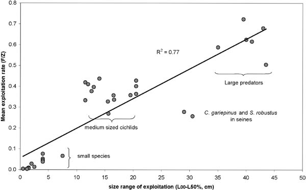
Exploitation rates are clearly clustered in three separate groups consisting respectively of large predators, medium sized cichlids and all the small species. The two outliers are C. gariepinus and S. robustus, caught in the seine nets. All small species are very lightly exploited (E< 0.1), the medium sized species seem fully exploited (0.3<E<0.5), whereas the largest species are over-exploited in terms of the long-term steady-state MSY (E>0.5) (Table 9). This trend is independent of gear category. All three gears are again sharing the three top positions in terms of exploitation levels: kutumpula for C. gariepinus, seines for H. vittatus, and gillnets for S. robustus. Interesting to note, is that even if effort were to be adjusted to the recommended exploitation levels for each gear category (Table 9), the overall long term improvement in yields would only be about 44 tonnes per year, which is less than two percent of the present yield.

TABLE 10. Summary of Thompson and Bell long term Yield predictions by species (all gears combined), by gear (all species combined) and for all species and all gears combined (multi-species, multigear analysis). To be able to interpret the results of this analysis only the eight species which had defined MSY’s within the range of simulated effort levels in the single-species, single-gear analysis were included, that is those with exploitation levels higher than 0.1. The top panel shows the results of each of the eight species based on all three gears combined, i.e. the overall “optimal” exploitation level (effort-factor) of these species compared to the present level with the present combination of gears. Also shown are the cohort analysis results (E-mean and F-mean) on the combined catches of each species in all gears. The middle panel presents the effort-factor estimates of each of the three gears based on all the eight species combined. The bottom panel presents the overall effort-factor, Present Yield and estimated MSY of the all the eight species in all three gears. Z = total mortality. Diff. % = percentage difference between the present estimated yield and the estimated MSY.

Only the three largest species (Clarias gariepinus, Hydrocynus vittatus and Serranochromis robustus) are biologically “overexploited” in terms of individual maximum yields in the combination of the three gears (Table 10). A reduction in fishing effort could therefore theoretically increase (marginally) the total yield for these species. However, optimizing the yield for H. vittatus by 15 percent with a reduction in effort of 40 percent will have no major effect on the total catch since the contribution of this species is limited to 25-30 tonnes per year. S. robustus catches could be optimized by 12 percent, but the fishing effort should then be reduced with 60 percent, and this would in turn cause a serious reduction in the catches of smaller species. By contrast, the remaining five species can all be submitted to a higher fishing pressure to increase yields, but again the effect would be rather small: an overall increase of effort of 30 percent, as suggested in the all gears, all species combination, would theoretically only improve the yields with around 2 percent. The overall conclusion from this analysis is that the yield obtained with the present combination of gears and effort is remarkably close to the potential long term MSY under steady state conditions.

5.3 Biomass-size distribution

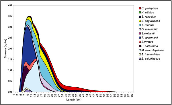
Based on the cohort analysis of the catches in the experimental gillnets (considered the least selective of the gears studied) a relative biomass-size structure of the main species caught in the Bangweulu swamp can be constructed (Figure 8). The small insectivorous and herbivorous species and individuals with a mode of 9-10 cm dominate the fish community and the biomass is characterized by a steep decline up to a size of around 30 cm. Although the large predators (C. gariepinus, H. vittatus and S. robostus) are the most heavily exploited (Table 10) these species are relatively abundant beyond 30 cm and cause the steep decline to taper off from this size. This could indicate that the larger sized specimen are relatively undisturbed by the present fishery, once grown in size beyond the selectivity range of the present exploitation pattern of the fishery.

FIGURE 8. Relative biomass (kg/ha) versus size (cm) of the 13 most common species in the Bangweulu swamps from cohort analysis on the experimental gillnet catches.

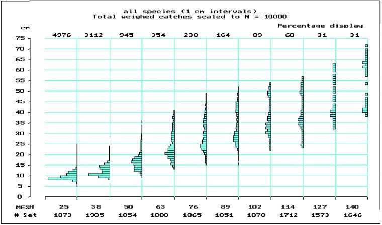
The biomass-size distribution in the Bangweulu swamps would explain the high frequency of small mesh sizes found in the Bangweulu fishery (Table 4). 90 percent of the gillnet catches in numbers are taken in mesh sizes smaller than 50 mm (Figure 9). These catches consist mainly of T. sparmanni and M. macrolepidotus, which are low to moderately exploited (Table 9).

FIGURE 9. Length frequency distributions and relative number of fish caught (on top, fraction of 10 000) of all species caught in the different mesh sizes of gillnets in Bangweulu swamps.

5.4 Overall yield estimates

Table 11 gives the contribution to the total yield for the three fishing methods studied. CPUE from data collected by fishermen (by method and mesh size) and Frame Survey figures on total numbers of fishing gear (by type and mesh size) were used to estimate yields. Total annual yield for the swamps in the gillnets, kutumpula and seines is estimated at an average of 2 828 tonnes per year for the period July 1994 to July 1996.

TABLE 11. Yield estimates (tonnes/year) for the Bangweulu swamps for the period July 1994 to July 1996 in the three gears studied, and the relative contribution of the eight species included in Thompson and Bell long term yield predictions to the total yield.

In an independent survey on the weirs (Chanda, 1998) this fishery was estimated to produce 6 260 tonnes in 1997, of which C. gariepinus alone contributed more than 2 000 tonnes. This means that the weir fishery produced more than twice the amount of the three other main methods combined. The weir fishery, which is the main method in the seasonal floodplains, is catching a broader size range and a larger proportion of small specimens, and is therefore the least selective of the main fishing methods in Bangweulu (Chanda, 1998; Table 4). In terms of species this fishery mainly targets Clarias gariepinus (35 percent), Tilapia rendalli (12 percent), Serranochromis angusticeps (11 percent), Marcusenius macrolepidotus (11 percent), and Serranochromis mellandi (9 percent) by weight respectively (Chanda, 1998). None of these species are overexploited according to this study (Table 10). For all four gears together, the swamps and floodplains are thus producing around 9 000 tonnes of fish per year, or about 59 percent of the whole Bangweulu fishery (Figure 3). This estimate is in close accordance to Bazigos, Grant and Williams (1975) who estimated that in 1973-1974 an average of 54 percent of the total yield for the Bangweulu fishery is produced by the swamps. Table 11 also indicates that the contribution of the eight selected species used in the Thompson and Bell long-term yield prediction accounted for 75 percent of the total yield of the three gear types studied. Thus the majority of the exploited stocks is taken into consideration. Though catch rates for the three methods in this analysis differ by a factor 10 to 25 (Table 11), the outcome of the daily catch of an individual fisherman appears to be remarkably similar for the three methods when considering the actual daily effort. A gillnet fisher usually owns 8 to 10 gillnets and he operates them on his own. This results in a catch rate between 6.9 and 8.6 kg for a gillnet fisher per day. Kutumpula fishers often team-up with colleagues to be able to enclose a larger area, but each of them uses his own net. This results in a catch rate of 9.6 kg per day for a Kutumpula fisher. Seine fishers have to employ three to four assistants to operate the seine. Usually the catch is shared between the owner and his assistants, resulting in a catch of between 4.4 and 5.5 kg per fisher. These are of course rough estimates and considerable differences will exist between fishers due to differences in quality of the fishing gear (state of maintenance) and the skills of fishermen.

5.5 Catch rates in Bangweulu compared with other African fisheries.

A comparison of catch rates from different other water bodies in Africa (Table 12) shows that in general the catch rates in Bangweulu are low in terms of weight, but high in terms of numbers compared to the other systems. It should be noted that the data from Lake Kariba are from an unfished locality (Zimbabwean side) and from an intensely fished area (Zambian side) (see also Kolding, Musando and Songore this volume, 2003). The CPUE by weight in the experimental multi-filament gillnets in Bangweulu is higher than in Lake Kariba (Zambian side) which is a heavily fished system, but lower than the heavily fished Lake Mweru and the unfished Zimbabwean side of Lake Kariba. The CPUE by number, however, is among the highest of all the other systems and correspondingly the mean weight of the fish, 30 g in the multi-filament nets, is the lowest. This demonstrates the small average size of the fish in Lake Bangweulu as already seen from the biomass-size distribution (Figure 8). Differences in mean size may not be directly comparable between a swamp and an open lake ecosystem. The Okavango Delta, however, should in many ways be an ecosystem comparable with the Bangweulu swamps and here the catch rates in the Lundgren nets are among the highest of the different systems. In contrast to Bangweulu, the Okavango Delta is very lightly exploited (Mosepele, 2000) and this could be a reason for the higher catch rates and higher mean weight. On the other hand, the Okavango River in Namibia is generally highly exploited, and here the catch rates are slightly lower than in the Bangweulu swamps, although the mean weights are higher (Table 12).

TABLE 12. Comparison of catch rates (mean ± SE) for different water bodies in Africa using similar experimental, monofilament (Lundgren) gillnets (42 x 1.5 m) and standardiszed multifilament experimental gillnets (45 x 2 m). Sources: Lutembwe, Mukungwa and Kang’ombe (Fjälling and Fürst, 1991). Kariba, Zimbabwian side (= unfished) (Karenge, 1992 and Sanyanga, 1996), Kariba, Zambian side (= fished) (Musando 1996), Lake Ziway (Gelchu 1999), Okavango Delta, Botswana (Mosepele 2000 and Mmopelwa unpublished), Khashm El-Girba (Salih 1994), Mweru-Luapula (van Zwieten and Kapasa, 1996), Okavango River, Namibia (Hay et al., 2000). As the CPUE is obtained with similar standardiszed gillnets (same twine, mesh sizes and gear area), the values are comparable as indices of the fish abundance in the different systems.