CHAPTER 6

Biodiversity assessment

In the context of this report, biodiversity refers to the plant diversity that can be observed by conventional means and without significant investment of effort for extended periods of time before the assessment. Essentially, it is understood here as the diversity that can be determined while undertaking simultaneously the morphometric measurements for biomass estimation and the field observations for land degradation assessment at the nested quadrat sites used for field sampling.

Measures of biodiversity at the level of species or populations are directed towards the attainment of an index of the number of species and their relative abundances within a given landscape. These indices are some of the most useful measures of biodiversity because species are more tangible and easier to study than communities or entire landscapes.

Typically, strategies for measuring biodiversity at this level involve protecting a single species. Nevertheless, this protection could help other species in different ways, such as species with similar habitat requirements, species with a large number of other species depending on it, or species with large area requirements (Noss, 1990). Therefore, ecologists use measures of the number of species or their relative abundances in order to address biodiversity from species diversity to the ecosystem level (Noss, 1999). The approach consists of broad habitat protection to benefit a wide range of species as ecosystems consist of the population of all species coexisting at a site. They also include the abiotic factors, which are interdependent with the biotic community.

Consequently, ecosystem diversity attempts to protect several species by preserving the habitat in which they live.

The relationship between the structure of the landscape and the diversity of the ecosystems present can be used to design mechanisms for the assessment of biodiversity at the landscape level. This could be of particular benefit to those assessment methods that employ remote-sensing techniques. Satellite image classification could then provide a useful spatial framework tool for collecting data at this level.

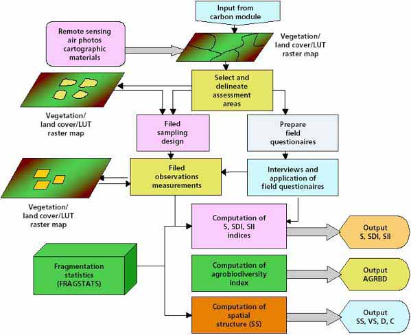
Classification of the landscape into vegetation types or landscape element types can also be used in order to provide a geographical framework for predicting the status of biodiversity of the landscape, provided that the variation of biodiversity measurements (e.g. species numbers, richness and abundance) within such units is much smaller than those between them. This is a precondition for the validity of any mapping units. Figure 23 illustrates the methodological steps for assessing biodiversity.

Remote sensing in the assessment of biodiversity

Satellite images provide almost the only source of reasonably continuous data on the reflectance properties of the ground and the ground cover. Such products can be used for the upscaling or interpolation of estimates or measures of diversity at specific sampling sites.

FIGURE 23 - Assessment of species diversity and agrobiodiversity of actual land use

Classification and mapping of land cover or vegetation types

A satellite image can help in interpreting differences in land cover and land use by exploiting the differences in reflectance of multiple spectral wavebands. For example, an FCC image, typically created using band 5: 1.55-1.75 nm (middle infrared), band 4: 0.76-0.90 nm (near infrared) and band 3: 0.63-0.69 nm (red) of Landsat TM7 imagery, could help in classifying land cover and land use. Every pixel of the FCC image is assigned a class of land cover or land feature, depending on the internal algorithms of the software for classification. This classification should be supervised by defining locations in the image where there is certainty of the corresponding land cover class. The classification from these training sites is expanded to the total of pixels in the image, creating a supervised classification and a map showing the spatial extent of land cover classes.

Indigenous knowledge of the local vegetation and its successional stages can prove invaluable in identifying vegetation types and suitable training sites for supervised classification. Exact location of the training sites on the ground can be achieved using a hand-held GPS unit. Training sites are identified and located for all identified vegetation types and subtypes. After trial and error, removing some unusable or redundant training areas, a total number that seems to achieve the best results in the classification should be determined.

In addition to the training areas, the six bands (TM 1, 2, 3, 4, 5 and 7) of Landsat TM7 imagery are used in the supervised classification in order to produce a vegetation raster map with several landscape element types (vegetation classes). The maximum likelihood algorithm is recommended for a supervised classification and for mapping the vegetation classes. The system calculates the statistical properties of the reflectance values for each cover type within each selected band, in this case for the six bands. The system then extrapolates the results, allocating each pixel of the image to the most appropriate class. After several trials to remove some of the bands, a final vegetation raster map is produced using red, near-infrared and middle-infrared bands (TM 3, 4 and 5), which achieve best results. In order to remove the speckle in the classified image, filters may have to be applied.

A supervised classification to produce a vegetation raster map is a relatively expensive exercise owing to the fieldwork component. Therefore, the use of an unsupervised classification can be explored as a less expensive option. The unsupervised classification does not require field support, it is used where there is minimal information about the classes to be recognized and separated in the image. Typically, the unsupervised classification can be considered as a preliminary classification, providing a first approximation to expected classes in the field. The classificatory algorithm used in the unsupervised classification groups data automatically, recalculating class means, and merging and splitting classes as required. The unsupervised classification assigns pixels to a specific number of classes in order to maximize their discrimination on the basis of reflectance values alone, in the number of bands used for classification. Therefore, the most difficult task in this type of classification is to determine the features corresponding to the resulting classes present on the ground.

The generated vegetation/land cover map from the multispectral classification of the satellite images can then be used as a geospatial framework for designing the sampling scheme and the distribution of quadrat sampling sites in the field. The mapping units provide the strata for reference in sampling.

Biodiversity indices

Several quantitative indices have been designed to provide information on the various aspects of plant diversity in landscapes. Table 13 lists some of those most widely used. However, it was necessary to introduce an ad-hoc designed index for agricultural diversity: the Agrobiodiversity Index (AgrBD). This can be calculated from: AgrBD = (S_D/S)T Dt, where S_D is the number of domesticated species in the total number of species S identified; Dt is the elapsed time between the beginning and end of the cropping cycle; and T is the number of consecutive years that the crop mix has been on a particular field or area. For 0 < AgrBD < 365, if T = 365 days. Thus, if AgrBD = 365, all biodiversity is agrobiodiversity.

TABLE 13 - Diversity indices for assessing plant diversity

* The Indices are cited in Magurran (1988).

Where: S = number of species; N = number of individuals; p_i = the proportion of individuals found in the i-th species; N_max = number of individuals in the most abundance species.

The various biodiversity indices (i.e. plant diversity in this context) can be used depending on the circumstances of the area under study and the incorporation of the nature of the diversity information required to monitor changes with changes in land use. For example, measures of plant diversity that are useful in cropland may not be so useful in the Amazon context. The indices from the list in Table 13 that were used for the case studies reported in this document were:

• species richness: number of species (S);

• Simpson Diversity Index;

• Shannon Diversity Index;

• agrobiodiversity (AgrBD).

The diversity inside a community is also known as “ a diversity”. To measure a diversity, species richness, Shannon Diversity Index and Simpson Diversity Index were used. Species richness is estimated with the total number of observed species. The Shannon Diversity Index is calculated by multiplying a species proportional abundance by the natural log of that number:

where p_i is the proportion of individuals found in the species “i”. This index assumes that individuals are sampled randomly from an infinite or very large population. Similarly, it supposes that all species are represented in the sample. The value of the Shannon Diversity Index usually falls between 1.5 and 3.5 and only rarely exceeds 4.5.

The Simpson Diversity Index is defined as the sum of squares of proportion abundance of each species:

As D increases, diversity decreases. Therefore, the Simpson Diversity Index is usually expressed as 1 -D or 1/D. Where 1 - D is used as the index, it ranges from 0 to 1, with values close to 1 showing a community of many species with equally low abundances while numbers close to 0 express fewer species with one of them clearly dominant.

The computation of the so-called spatial structure index makes sense in situations where there are significant levels of vegetation canopy, and where these vertical structures appear to influence directly the diversity of other species, whether plants or animals (e.g. Amazon rainforest). In the case studies used to illustrate this method, the spatial structure index was not computed.

Field sampling,measurement and data processing for biodiversity

Field survey and sampling need to be undertaken in order to estimate the biological composition (plant diversity) of several landscape element types (vegetation types). As this survey is conducted simultaneously with the biomass measurements and the land degradation assessments, the sampling units are essentially the same. The sampling design and the distribution of the sampling sites on the ground are also identical.

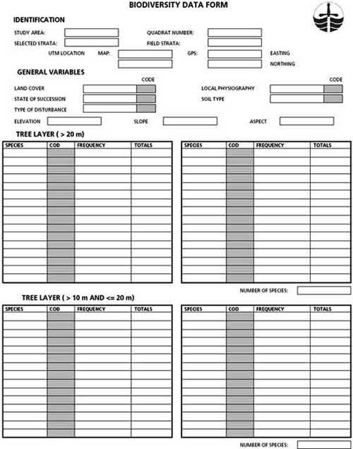
The sample unit on the ground consists of a quadrat of 10 × 10 m in which the number of trees by species must be recorded. Where there are clearly distinguishable canopy layers, these can be sampled separately to facilitate the identification of species. For every canopy layer considered, the identification of species should proceed. For example, in a first canopy layer, trees that are 20 m or higher can be identified and counted. A second layer should consider trees between 10 and 20 m high. A third layer should consider trees of less than 10 m, and so on. Every 10 × 10 m quadrat contains a nested subquadrat of 5 × 5 m for sampling shrubs taller than 1 m. A further nested subquadrat of 1 × 1 m is used for sampling the dominant herbs, and all the tree regrowth and shrub species less than 1 m high. Therefore, trees, shrubs and dominant herbs that fall within the sampling quadrats characterize the biological composition of plants in the study area. Sampling sites should be georeferenced using a GPS. This will allow the digitizing of all sample site locations, after being validated, for entry into a spreadsheet or a database. At each of the sampling quadrats, plant species are identified and counted using special field forms. These forms should be designed ahead of the fieldwork and should be used for recording field data in the event of having no means of direct digital recording (i.e. digital data logger). The example in Figure 24 illustrates a field data form for recording biodiversity data.

FIGURE 24 - A field data form for recording biodiversity data

Identification of species

One of the most difficult tasks during fieldwork could be the identification of species on the ground.

A major constraint in practice is the impossibility to collect plants with all the plant morphology components needed for identification in a herbarium, and to have available the time and effort that this requires. It is highly recommended that a member of the field team be a botanist, plant taxonomist or forest taxonomist, who could at least make an approximate identification of difficult species, thereby minimizing the amount of plant collection required for later identification in the herbarium or laboratory.

On the other hand, where no member of the field team has the required expertise for plant identification, a useful strategy is to benefit from indigenous knowledge by engaging the help of knowledgeable local people. These are people who are plant experts or have been working in the area long enough to have the ability to identify species using local names. Published work describing the vegetation of the study area should be reviewed as it may also prove extremely valuable.

Estimating sample size

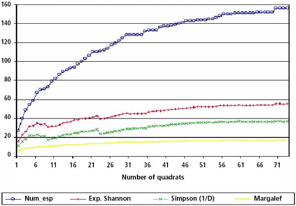
For the purposes of identifying the optimal sample size, an interactive approach can be followed. Pielou’s pooled quadrat method (Magurran, 1988) can be used to calculate the number of samples needed in the landscape in order to produce reliable estimates of the status of biodiversity in the area. The method consists of taking a sample of one quadrat at a time, and calculating incrementally and iteratively the diversity values (indices) in the quadrats entered. The number of samples is then increased to 2, 3 and 4 quadrats, and so on, until all the quadrats sampled so far are accounted for. A fresh set of diversity values is calculated with the pooled data each time. The calculated biodiversity indices should be plotted as they emerge from calculations from the current field samples against the total number of samples used in the calculation. This should allow for monitoring the number of samples after which gains in the values of the indices are negligible or nil (i.e. the curve of the index becomes asymptotic to the axis of the number of samples). Figure 25 illustrates this procedure.

FIGURE 25 - Graph of plant diversity indices against number of sampling quadrat sites to determine the number of sites needed

In practice, as the sampling sites are multipurpose sites, the final number of sampling sites will be a compromise between the factors mentioned above and considerations related to biomass estimation and land degradation assessment.

Biodiversity database development

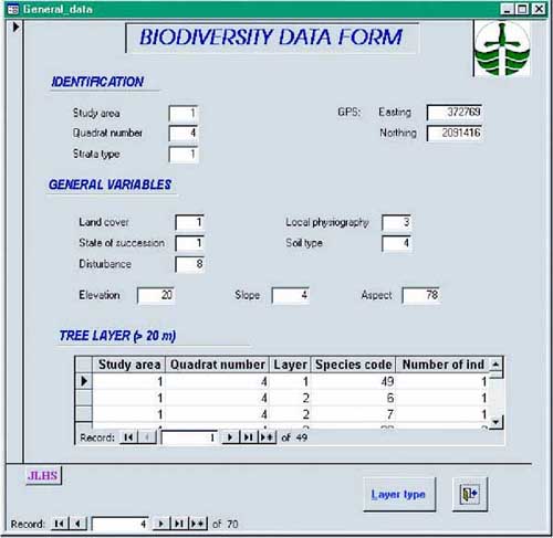
For the purpose of systematically storing and processing the field data in an almost simultaneous fashion as they are entered, in addition to retrieving diversity data, a dedicated database system was developed and implemented by customizing a commercially available DBMS (ACCESS). All field data were input, processed and validated into the customized program. Although the system was implemented to recover all indices presented in Table 13, which can be calculated by quadrat as well as by trees and shrub layers, a user able to manipulate standard query language could make any query and consultation to the database. The customized program also allows users to enter, delete and update information on quadrats and species. Figure 26 illustrates the data entry screen of the database.

Three standard biodiversity indices, namely: species richness, Shannon Diversity Index, and Simpson Diversity Index (Magurran, 1988; Whittaker, 1972), as well as Margalef, species evenness, Reciprocal Simpson and Reciprocal Berger-Parker indices, can be computed almost instantaneously by using the customized database.

FIGURE 26 - Customized biodiversity database (plants)

Geospatial framework for upscaling and interpolating diversity indices

The raster map of land cover or vegetation classes, which results in the so-called “landscape element types” after the satellite image multispectral classification, provides strata useful as a frame for sampling. It can also be useful for upscaling and the interpolation of diversity indices. The distinct classes of pixels that can form clusters and mapping units, or can be converted to polygons in vector format, are the units for upscaling. Both polygons and raster mapping units can be used as a geospatial framework to upscale and interpolate the computed indices of plant biodiversity. The properties of internal homogeneity or uniformity of such mapping units can be exploited to serve in the upscaling or spatial extrapolation or interpolation of plant diversity indices computed at specific locations (point data).

Uniformity index to assess the homogeneity of mapping units

As the usefulness of the mapping units for upscaling will depend directly on their internal homogeneity, this needs to be tested. In order to provide an indicator of the degree of internal uniformity of each of the classes on the plant diversity indices that are calculated from quadrat sampling data, a uniformity index can be computed as a measure of the goodness of the classification in partitioning spatial variability and creating strata (classes) that can be used for interpolation. The uniformity index is calculated by subtracting the relative variance from 1. The relative variance is a ratio of the within-class variance to total sample variance. When the value of the index is close to 1, the mapped class boundaries are very meaningful in terms of partitioning the variability of plant diversity indices across the landscape. The within-class variance is considerably smaller than the total variance, indicating that the classes are relatively homogeneous. This could also be viewed as a strong relationship between the spatial distribution of plant diversity indices and the boundaries of the mapped classes. The species composition of the vegetation classes can be separated by such boundaries of the vegetation classes identified in the field. Therefore, the classes are useful for discriminating plant composition of each landscape element type. The equation for calculating the uniformity index (U) is:

where: is the within-class variance, and is the total variance.

Assessing map accuracy of the vegetation map produced

The randomly selected field samples of vegetation from quadrat sites can be used for assessing the accuracy of the landscape classification. These samples can be used to estimate plant diversity at field level and to test the accuracy of the classes derived from satellite image interpretation. The assessment of the accuracy of the classification can be based on two procedures: (i) overall accuracy; and (ii) Cohen’s Kappa statistic. These are the most common techniques for assessing the agreement between classes in the map and classes on the ground. The overall accuracy of the classified image can be computed by dividing the total number of correctly classified sampling quadrats by the total number of sampling quadrats. The overall accuracy (AC_o) can be written as:

where: is the total number of sampling quadrats classified correctly, and is the total number of reference sampling quadrats placed in the field.

The Cohen’s Kappa statistic (Campbell, 1987) measures the excess of agreement between map and reality over the level of agreement that would have been obtained by chance alone. The Kappa (K) coefficient will equal 1 if there is perfect agreement, whereas 0 is what would be expected by total chance alone. The equation of the Kappa statistic can be written as:

where: d is the overall value for percentage correct; q is the estimate of the chance agreement to the observed percentage correct (these values are calculated using number of cases expected in diagonal cells by chance, and are drawn from some form of contingency table); and N is the total of number of cases.

A value of the Kappa statistic of 0.5 would imply that the mapping units predict reality with 50 percent reliability. Thus, the map is not very much better than chance.

Assessments of both internal homogeneity of mapping units (uniformity index) and map accuracy (Cohen’s Kappa) are essential to determine the usefulness of the mapped classes for upscaling and interpolation of diversity indices.

Relating multispectral vegetation classes to biodiversity indices

The main practical objective of linking field quadrat measurements of plant diversity to vegetation classes, as derived from multispectral satellite image classification, is to explore the relationships between mapped boundaries of classes on the image and the spatial distribution of indices of plant diversity. Finding a strong association between them would allow for exploiting the map of vegetation classes as a mechanism for upscaling measurements on the ground to an entire landscape. This process can be considered as a typical case of spatial interpolation of point data (quadrat sites). The approach adopted in this report for the upscaling process uses the multispectral class boundaries as domain limits within which the diversity indices values are interpolated. Hernandez-Stefanoni and Ponce-Hernandez (2003) provide a description of the procedure.

It is recognized that other important techniques for spatial interpolation (e.g. geostatistical techniques, distance functions, and bicubic splines) are available and should be attempted, provided favourable conditions of number of samples (point data) and spatial structure in the diversity indices exist. However, this section concentrates on exploring the virtues of mapped vegetation classes to indirectly stratify and map plant diversity indices, and on how to use such a spatial framework for upscaling biodiversity measurements to the landscape scale.

Thus, in order to estimate the biological composition of the entire studied area based on the classification derived from the multispectral satellite image, two steps need to be considered. First, several diversity indices can be calculated by vegetation type (mapping unit) by pooling all the field quadrats of every vegetation class, as derived from the multispectral classification. Second, this report adopted the approach suggested by Burrough and McDonnell (1998) to spatial prediction based on classes. This approach essentially makes use of the classes as the mechanism for interpolating values of the class attributes to the entire area covered by each class. The approach assumes, in this case, that diversity values within vegetation classes are significantly lower than those between them. That is to say, that the within-class variability of the attribute needs to be confirmed as substantially smaller (i.e. internal homogeneity) than the variability across classes before a class can be used as a mechanism for extending the values of its attributes to all locations within the class.

A standard ANOVA can compute the variances required for testing the contributions of quadrats, vegetation types and the residual error to the total variability of the calculated diversity indices in the area. The ANOVA to be undertaken could use themodel:

where: Y_ij is the number of species or abundance in the j-th quadrat within the i-th vegetation type; m is the general mean of all vegetation types; vt_i is the effect of i-th vegetation type; and e_ij is the error in the j-th quadrat within the i-th vegetation type orsubtype.

The one-factor ANOVA model can test for significant differences in the diversity of plants across vegetation classes. Thus, through the ANOVA, a comparison can be made between the mean of the number of species by quadrat (that is the species richness in 100 m²), and the mean values of the exponential Shannon Diversity Index and Reciprocal Simpson Index (1/D) by quadrat, among the vegetation types. The Least Significant Difference test (Tabachnick and Fidell, 1996) can be used to determine whether there are significant differences among classes.

As described by Hernandez-Stefanoni and Ponce-Hernandez (2001), a number of assumptions are necessary in order to use vegetation classes and their mapped spatial extents as a reliable mechanism for making predictions of biodiversity values. First, the values of diversity data should be random and not spatially continuous. This means that the value of the diversity indices should be independent of the location inside each polygon (landscape element type). Second, the variance of diversity data within vegetation classes should be small if not homogeneous. Third, all diversity values should be distributed normally, in the probabilistic sense. Finally, all spatial changes should take place at boundaries in a relatively sharp manner (Burrough and McDonnell, 1998). For testing the assumptions of normality of the data, the Komolgorov-Smirnov test can be used. Levene’s test could be used for testing the homogeneity of variance among vegetation classes. Thus, randomness and independence can be dealt with only indirectly through the tests indicated above and through the ANOVA tests. It is presumed that the plant diversity indices are quasi-stationary over space, which is characteristic of transition phenomena, accounting for small within-class variations.

Mapping biodiversity indices

The procedures discussed above provide a range of techniques that can be used under different circumstances of data and variability to map out the spatial extent of plant diversity indices and to obtain a display of the spatial distribution of the diversity of plants in the area of concern.

Using mapping unit polygons as interpolants is the simplest mapping method. This method enables use of GIS functionality. The process would consist essentially of calculating a particular diversity index from within-class pooled data on, and attributing that value to, the polygon from which the quadrat data were pooled. Polygon attribute assignment functions that are used in this situation are a standard function in any GIS software.

Spatial interpolation with block kriging requires that a clear spatial structure be found in the semi-variogram of the diversity index, and that anisotropies are accounted for. Typically, this technique would be demanding in terms of the number of sample sites (point data) required for an optimal interpolation, but it would not use the vegetation classes mapped out with the multispectral classification. The map resulting from block kriging would be a raster map of the diversity index.

Other spatial interpolation methods, such as bicubic splines (an exact interpolator), would make fewer demands on the number of sampling sites but would create a smoothing effect. This method does not use the vegetation classes from the multispectral classification. A “gridding” method has to be chosen where other interpolation packages that do not use block kriging or bicubic splines are used. Typically, this “gridding” or interpolation method is some form of distance function moving average.